Thus far, we’ve explored score models in the context of 1D data. This is intentional! By working out the core ideas in a single dimension, we can more easily reason about what actually is happening – humans are, after all, very good at thinking in 1D. In effect, we eliminate the cognitive load that comes with thinking multi-dimensionally. Through this, the framework of how to think about how to use score models to generate data is quite clear. Our ingredients are:
Data,
A trainable model that can approximate the score of our data (implying that yes, we will train that model!), and
A procedure for noising up data and reversing that process to re-generate new data.
Alas, however, the world of data that inhabits our world is rarely just 1D. More often than not, the data that we will encounter is going to be multi-dimensional. To exacerbate the matter, our data are also oftentimes discrete and not continuous, such as text, protein sequences, and more. Do the ideas explored in 1D generalize to multiple dimensions?1 In this notebook, I want to show how we can generalize from 1D to 2D. (With a bit of hand-waving, I’ll claim at the end that this all works in n-dimensions too!)
6.1 Data: 2D Gaussians and Half Moons
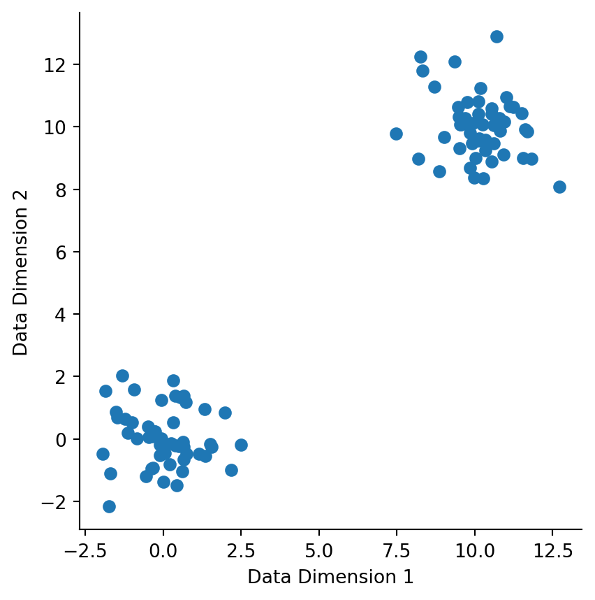
In this anchoring example, we will explore how to train a score model on both the half-moons dataset and a simple 2D Gaussian. For ease of presentation, the code (as executed here) will only use the half-moons dataset but one flag at the top of the cell below, MOONS = True, can be switched to MOONS = False to switch to the 2D Gaussian dataset.
Code
import jax.numpy as np from jax import random import matplotlib.pyplot as plt from sklearn.datasets import make_moons, make_circlesimport seaborn as sns# CHANGE THIS FLAG TO FALSE TO RUN CODE WITH 2D MIXTURE GAUSSIANS.DATA ="gaussians"N_DATAPOINTS =100if DATA =="moons": X, y = make_moons(n_samples=N_DATAPOINTS, noise=0.1, random_state=99)# Scale the moons dataset to be of the same scale as the Gaussian dataset. X = X *10elif DATA =="circles": X, y = make_circles(n_samples=N_DATAPOINTS, noise=0.01, factor=0.2, random_state=99) X = X *10else: key = random.PRNGKey(55) k1, k2 = random.split(key, 2) loc1 = np.array([0., 0.]) cov1 = np.array([[1., 0.], [0., 1.]]) x1 = random.multivariate_normal(k1, loc1, cov1, shape=(int(N_DATAPOINTS /2),)) loc2 = np.array([10., 10.]) cov2 = cov1 x2 = random.multivariate_normal(k2, loc2, cov2, shape=(int(N_DATAPOINTS /2),)) X = np.concatenate([x1, x2])plt.scatter(*X.T)plt.gca().set_aspect("equal")plt.xlabel("Data Dimension 1")plt.ylabel("Data Dimension 2")sns.despine()
Figure 6.1: Sample synthetic data that we will be working with.
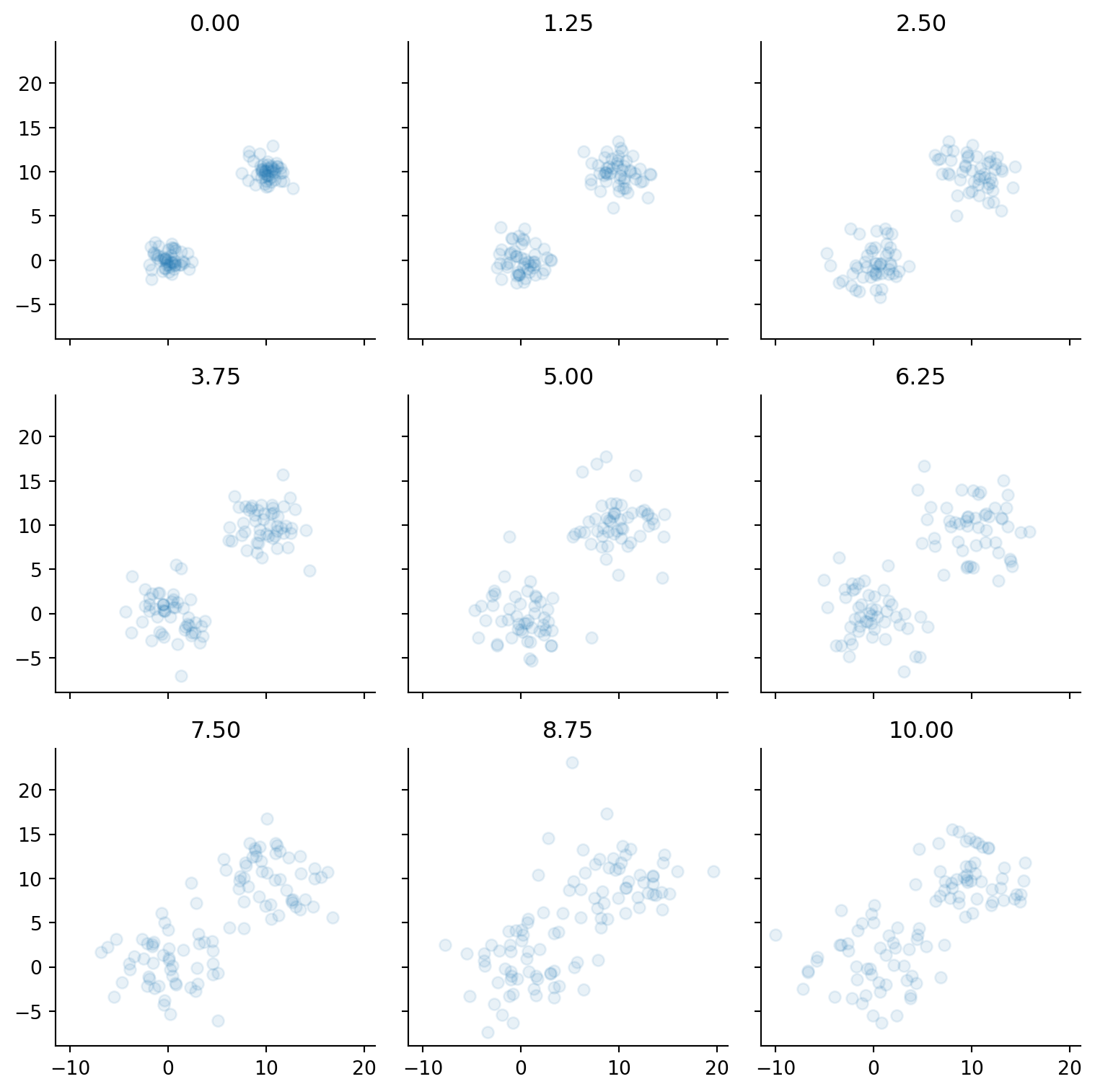
6.2 Add noise to data
Next we noise up the data. Strictly speaking with a constant drift term, we need only parameterize our diffusion term using t (time) and don’t really need to use diffrax’s SDE capabilities. We can noise up data by applying a draw from an isotropic Gaussian with covariance equal to the time elapsed.
Code
from jax import vmapfrom functools import partialimport seaborn as sns def noise_batch(key, X: np.ndarray, t: float) -> np.ndarray:"""Noise up one batch of data. :param x: One batch of data. Should be of shape (1, n_dims). :param t: Time scale at which to noise up. :returns: A NumPy array of noised up data. """if t ==0.0:return X cov = np.eye(len(X)) * treturn X + random.multivariate_normal(key=key, mean=np.zeros(len(X)), cov=cov)def noise(key, X, t): keys = random.split(key, num=len(X))return vmap(partial(noise_batch, t=t))(keys, X)from jax import random fig, axes = plt.subplots(figsize=(8, 8), nrows=3, ncols=3, sharex=True, sharey=True)ts = np.linspace(0.001, 10, 9)key = random.PRNGKey(99)noise_level_keys = random.split(key, 9)noised_datas = []for t, ax, key inzip(ts, axes.flatten(), noise_level_keys): noised_data = noise(key, X, t) noised_datas.append(noised_data) ax.scatter(noised_data[:, 0], noised_data[:, 1], alpha=0.1) ax.set_title(f"{t:.2f}")noised_datas = np.stack(noised_datas)sns.despine()plt.tight_layout()
Figure 6.2: Synthetic data at different noise scales.
As a sanity-check, we should ensure that noised_data’s shape is (time, batch, n_data_dims):
noised_datas.shape
(9, 100, 2)
Indeed it is!
6.3 Score model definition
Now, we can set up a score model to be trained on each time point’s noised-up data. Here, we are going to use a feed forward neural network. The neural network needs to accept x and t; as with the previous chapter, we will be using a single neural network that learns to map input data and time to the approximated score function.
from score_models.models.sde import SDEScoreModel
If you are curious, you can see how the SDEScoreModel class is defined below.
from inspect import getsourceprint(getsource(SDEScoreModel))
class SDEScoreModel(eqx.Module):
    """Time-dependent score model.

    We choose an MLP here with 2 inputs (`x` and `t` concatenated),
    and output a scalar which is the estimated score.
    """

    mlp: eqx.Module

    def __init__(
        self,
        data_dims=2,
        width_size=256,
        depth=2,
        activation=nn.softplus,
        key=random.PRNGKey(45),
    ):
        """Initialize module.

        :param data_dims: The number of data dimensions.
            For example, 2D Gaussian data would have data_dims = 2.
        :param width_size: Width of the hidden layers.
        :param depth: Number of hidden layers.
        :param activation: Activation function.
            Should be passed in uncalled.
        :param key: jax Random key value pairs.
        """
        self.mlp = eqx.nn.MLP(
            in_size=data_dims + 1,  # +1 for the time dimension
            out_size=data_dims,
            width_size=width_size,
            depth=depth,
            activation=activation,
            key=key,
        )

    @eqx.filter_jit
    def __call__(self, x: np.ndarray, t: float):
        """Forward pass.

        :param x: Data. Should be of shape (1, :),
            as the model is intended to be vmapped over batches of data.
        :param t: Time in the SDE.
        :returns: Estimated score of a Gaussian.
        """
        t = np.array([t])
        x = np.concatenate([x, t])
        return self.mlp(x)
The key design choice here is that time t is made part of the MLP’s input by concatenation with x.
As always, we need a sanity-check that the model’s forward pass works:
from functools import partialfrom jax import vmap model = SDEScoreModel(data_dims=2, depth=3)t =3.0X_noised = noise(key, X, t)out = vmap(partial(model, t=t))(X_noised)out.shape
(100, 2)
Because the shape is correct, we can be confident in the forward pass of the model working correctly.
6.4 Loss function
Now, we need the score matching loss function; it is identical to the one we used in the previous chapter.
from score_models.losses import joint_sde_score_matching_loss
Let’s make sure that the loss function works without error first. Once again, this is a good practice sanity check to perform before we
model = SDEScoreModel(data_dims=2)joint_sde_score_matching_loss(model, noised_datas, ts=ts)
Array(1.3476348, dtype=float32)
As a sanity-check again, let us make sure that we can take the gradient of the loss function as well. To do so, we will use Equinox’s filter_value_and_grad, which is a fancy version of JAX’s value_and_grad that ensures that we calculate value_and_grad only on array-like arguments.
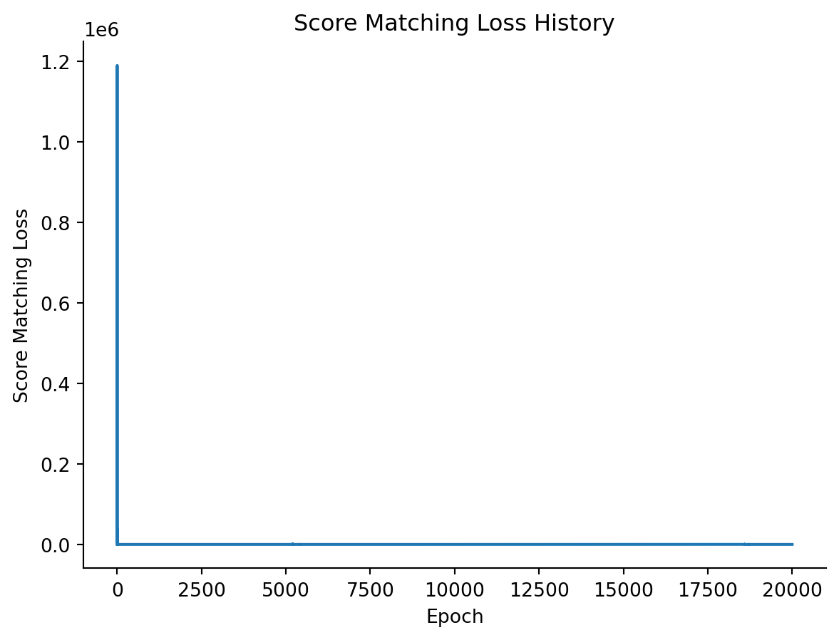
Let’s plot the losses so we can have visual confirmation that we have trained the model to convergence.
Code
plt.plot(loss_history)plt.xlabel("Epoch")plt.ylabel("Score Matching Loss")plt.title("Score Matching Loss History")sns.despine()
{#fig-training-loss· width=589 height=449}
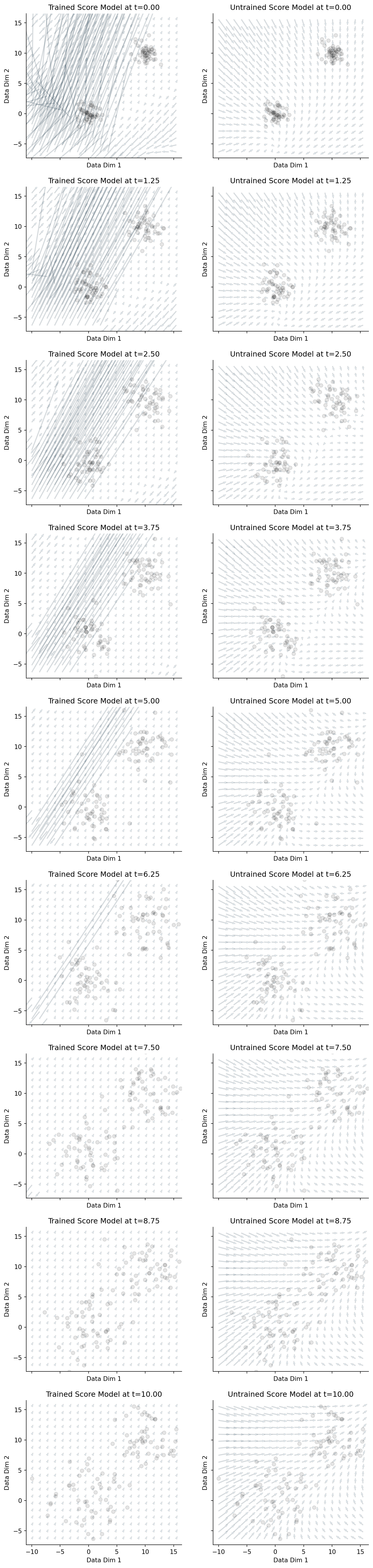
6.6 Visualize gradient field
In this particular case, because we have 2D data, one way of confirming that we have trained the model correctly is to look at the gradient field given by our trained score model. We will compare a trained model (on the left) to an untrained model (on the right). We should see that the gradient field points to the direction of highest data density,
Figure 6.3: Gradient field of trained vs. untrained models at varying time points (corresponding to different noise scales).
Notice how the gradient field on the right half of Figure 6.3 consistently ignores the density of data, whereas the gradient field on the left half of Figure 6.3 consistently points towards areas of high density.
6.7 Probability Flow ODE
With the gradient fields confirmed to be correct, we can set up the probability flow ODE.
We need a constant drift term, a time-dependent diffusion term, and finally, the updated score model inside there.
def constant_drift(t, y, args):"""Constant drift term."""return0def time_dependent_diffusion(t, y, args):"""Diffusion term that increases with time."""return t * np.eye(2)def reverse_drift(t: float, y: float, args: tuple): f = constant_drift(t, y, args) # always 0, so we can, in principle, take this term out. g = time_dependent_diffusion(t, y, args) s = updated_score_model(y, t)# Extract out the diagonal because we assume isotropic Gaussian noise is applied.return f -0.5* np.diagonal(np.linalg.matrix_power(g, 2)) * sfrom diffrax import ODETerm, Tsit5, SaveAt, diffeqsolveclass ODE(eqx.Module): drift: callabledef__call__(self, ts: np.ndarray, y0: float): term = ODETerm(self.drift) solver = Tsit5() saveat = SaveAt(ts=ts, dense=True) sol = diffeqsolve( term, solver, t0=ts[0], t1=ts[-1], dt0=ts[1] - ts[0], y0=y0, saveat=saveat )return vmap(sol.evaluate)(ts)
Now, let’s plot the probability flow trajectories from a random sampling of starter points.
from IPython.display import HTMLHTML(animation.to_jshtml())
Figure 6.4: Probability flow ODE and trajectories from a variety of randomly-chosen starting points. Circles mark the starting location, while diamonds mark the ending location of each trajectory.
As we can see in Figure 6.4, with an (admittedly not so) random selection of starter points, we can run the probability flow ODE in reverse time to get data coordinates that are distributed like our original starter data… without knowing the original data generating distribution! This is the whole spirit of score-based models, and in this chapter, we explored how to make that happen in a non-trivial 2D case. In principle, we could run with any kind of numerical data, such as images (where the original application of score models was done), or numerically embedded text (or protein sequences) from an encoder-decoder pair’s encoder module.
Of course, yes – this is a rhetorical question – and the more important point here is figuring out what we need to do to generalize beyond 1D.↩︎
 {#fig-training-loss· width=589 height=449}