%load_ext autoreload
%autoreload 2
%matplotlib inline
%config InlineBackend.figure_format = 'retina'

Neural Networks from Scratch

In this chapter, we are going to explore differential computing in the place where it was most highly leveraged: the training of neural networks. Now, as with all topics, to learn something most clearly, it pays to have an anchoring example that we start with.

In this section, we'll lean heavily on linear regression as that anchoring example. We'll also explore what gradient-based optimization is, see an elementary example of that in action, and then connect those ideas back to optimization of a linear model. Once we're done there, then we'll see the exact same ideas in action with a logistic regression model, before finally seeing them in action again with a neural network model.

The big takeaway from this chapter is that basically all supervised learning tasks can be broken into:

model
loss
optimizer

Hope you enjoy it! If you're ready, let's take a look at linear regression.

import jax.numpy as np
from jax import jit
import numpy.random as npr
import matplotlib.pyplot as plt
from ipywidgets import interact, FloatSlider
from pyprojroot import here

Linear Regression

Linear regression is foundational to deep learning. It should be a model that everybody has been exposed to before in school.

A humorous take I have heard about linear models is that if you zoom in enough into whatever system of the world you're modelling, anything can basically look linear.

One of the advantages of linear models is its simplicity. It basically has two parameters, one explaining a "baseline" (intercept) and the other explaining strength of relationships (slope).

Yet one of the disadvantages of linear models is also its simplicity. A linear model has a strong presumption of linearity.

NOTE TO SELF: I need to rewrite this introduction. It is weak.

Equation Form

Linear regression, as a model, is expressed as follows:

$y = wx + b$

Here:

The model is the equation, $y = wx + b$ .
$y$ is the output data.
$x$ is our input data.
$w$ is a slope parameter.
$b$ is our intercept parameter.
Implicit in the model is the fact that we have transformed $y$ by another function, the "identity" function, $f(x) = x$ .

In this model, $y$ and $x$ are, in a sense, "fixed", because this is the data that we have obtained. On the other hand, $w$ and $b$ are the parameters of interest, and we are interested in learning the parameter values for $w$ and $b$ that let our model best explain the data.

Make Simulated Data

To explore this idea in a bit more depth as applied to a linear regression model, let us start by making some simulated data with a bit of injected noise.

Exercise: Simulate Data

Fill in w_true and b_true with values that you like, or else leave them alone and follow along.

from dl_workshop.answers import x, w_true, b_true, noise

# exercise: specify ground truth w as w_true.
# w_true = ...

# exercise: specify ground truth b as b_true
# b_true = ...


# exercise: write a function to return the linear equation
def make_y(x, w, b):
    """Your answer here."""
    return None

# Comment out my answer below so it doesn't clobber over yours.
from dl_workshop.answers import make_y

y = make_y(x, w_true, b_true)

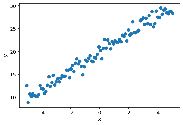
# Plot ground truth data
plt.scatter(x, y)
plt.xlabel('x')
plt.ylabel('y');

/home/runner/work/dl-workshop/dl-workshop/src/dl_workshop/answers.py:34: TqdmExperimentalWarning: Using `tqdm.autonotebook.tqdm` in notebook mode. Use `tqdm.tqdm` instead to force console mode (e.g. in jupyter console)
  from tqdm.autonotebook import tqdm
WARNING:absl:No GPU/TPU found, falling back to CPU. (Set TF_CPP_MIN_LOG_LEVEL=0 and rerun for more info.)

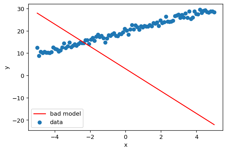
Exercise: Take bad guesses

Now, let's plot what would be a very bad estimate of $w$ and $b$ . Replace the values assigned to w and b with something of your preference, or feel free to leave them alone and go on.

# Plot a very bad estimate
w = -5  # exercise: fill in a bad value for w
b = 3   # exercise: fill in a bad value for b
y_est = w * x + b  # exercise: fill in the equation.
plt.plot(x, y_est, color='red', label='bad model')
plt.scatter(x, y, label='data')
plt.xlabel('x')
plt.ylabel('y')
plt.legend();

Regression Loss Function

How bad is our model? We can quantify this by looking at a metric called the "mean squared error". The mean squared error is defined as "the average of the sum of squared errors".

"Mean squared error" is but one of many loss functions that are available in deep learning frameworks. It is commonly used for regression tasks.

Loss functions are designed to quantify how bad our model is in predicting the data.

Exercise: Mean Squared Error

Implement the mean squred error function in NumPy code.

def mse(y_true: np.ndarray, y_pred: np.ndarray) -> float:
    """Implement the function here"""

from dl_workshop.answers import mse

# Calculate the mean squared error between 
print(mse(y, y_est))

702.42755

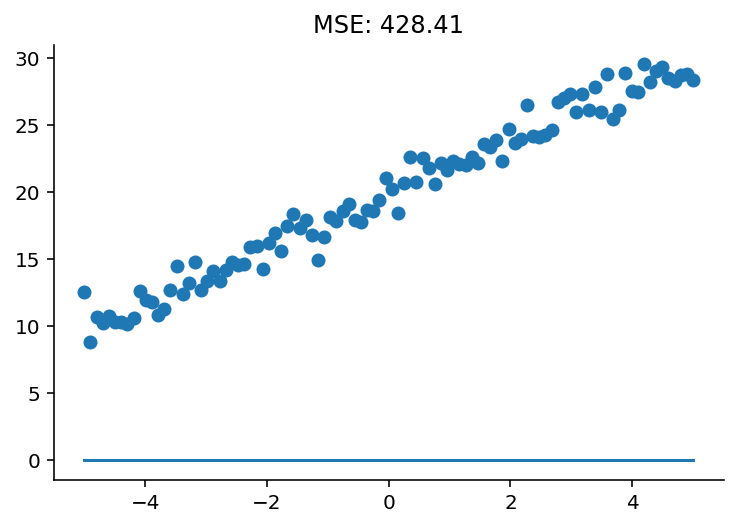
Activity: Optimize model by hand.

Now, we're going to optimize this model by hand. If you're viewing this on the website, I'd encourage you to launch a binder session to play around!

import pandas as pd
from ipywidgets import interact, FloatSlider
import seaborn as sns

@interact(w=FloatSlider(value=0, min=-10, max=10), b=FloatSlider(value=0, min=-10, max=30))
def plot_model(w, b):
    y_est = w * x + b
    plt.scatter(x, y)
    plt.plot(x, y_est)
    plt.title(f"MSE: {mse(y, y_est):.2f}")
    sns.despine()

Loss Minimization

As you were optimizing the model, notice what happens to the mean squared error score: it goes down!

Implicit in what you were doing is gradient-based optimization. As a "human" doing the optimization, you were aware that you needed to move the sliders for $w$ and $b$ in particular directions in order to get a best-fit model. The thing we'd like to learn how to do now is to get a computer to automatically perform this procedure. Let's see how to make that happen.