%load_ext autoreload
%autoreload 2
%matplotlib inline
%config InlineBackend.figure_format = 'retina'

Gaussian mixture model-based clustering

In this notebook, we are going to take a look at how to cluster Gaussian-distributed data.

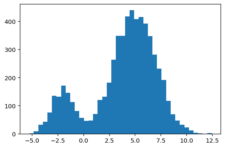
Imagine you have data that are multi-modal, something that looks like the following:

import jax.numpy as np
from jax import random
import matplotlib.pyplot as plt

weights_true = np.array([1, 5])  # 1:5 ratio
locs_true = np.array([-2., 5.])  # different means
scale_true = np.array([1.1, 2])  # different variances

base_n_draws = 1000
key = random.PRNGKey(100)

k1, k2 = random.split(key)

draws_1 = scale_true[0] * random.normal(k1, shape=(base_n_draws * weights_true[0],)) + locs_true[0]
draws_2 = scale_true[1] * random.normal(k2, shape=(base_n_draws * weights_true[1],)) + locs_true[1]
data_mixture = np.concatenate([draws_1, draws_2])
plt.hist(data_mixture, bins=40);

WARNING:absl:No GPU/TPU found, falling back to CPU. (Set TF_CPP_MIN_LOG_LEVEL=0 and rerun for more info.)

Likelihoods of Mixture Data

We might look at this data and say, "I think there's two clusters of data here." One that belongs to the left mode, and one that belongs to the right mode. By visual inspection, the relative weighting might be about 1:3 to 1:6, or somewhere in between.

What might be the "data generating process" here?

Well, we could claim that when a data point is drawn from the mixture distribution, it could have come from either of the modes. By basic probability logic, the joint likelihood of observing the data point is:

The likelihood that the datum came from the left Gaussian, times the probability of drawing a number from the left Gaussian, plus...
The likelihood that the datum came from the right Gaussian, times the probability of drawing a number from the right Gaussian.

Phrased more generally:

The sum over "components $j$ of the likelihood that the datum $x_i$ came from Gaussian $j$ with parameters $\mu_j, \sigma_j$ times the likelihood of observing a draw from component $j$ ."

In math, we would need to calculate:

$\sum_j P(x_i|\mu_j, \sigma_j) P(\mu_j, \sigma_j|w_j) P(w_j)$

Now, we can make the middle term $P(\mu_j, \sigma_j|w_j)$ is always 1, by assuming that the $\mu_j$ and $\sigma_j$ chosen are always fixed given the component weight chosen. The expression then simplifies to:

$\sum_j P(x_i|\mu_j, \sigma_j) P(w_j)$

Log Likelihood of One Datum under One Component

Because this is a summation, let's work out the elementary steps first.

from dl_workshop.gaussian_mixture import loglike_one_component

loglike_one_component??

The summation here is because we are operating in logarithmic space.

You might ask, why do we use "log" of the component scale? This is a math trick that helps us whenever we are doing computations in an unbounded space. When doing gradient descent, we can never guarantee that a gradient update on a parameter that ought to be positive-only will give us a positive number. Thus, for positive numbers, we operate in logarithmic space.

We can quickly write a test here. If the component probability is 1.0, the component $\mu$ is 0, and the observed datum is also 0, it should equal to the log-likelihood of 0 under a unit Gaussian.

from jax.scipy import stats

our_test = loglike_one_component(
    component_weight=1.0, 
    component_mu=0., 
    log_component_scale=np.log(1.), 
    datum=0.)

ground_truth = (
    stats.norm.logpdf(x=0, loc=0, scale=1)
)

our_test, ground_truth

(DeviceArray(-0.9189385, dtype=float32),
 DeviceArray(-0.9189385, dtype=float32))

Log Likelihood of One Datum under All Components

Now that we are done with the elementary computation of one datum under one component, we can vmap the log-likelihood calculation over all components, thereby giving us the loglikelihood of a datum under any of the possible given components.

Firstly, we need a function that normalizes component weights to sum to 1. This is enforced just in case during the gradient descent procedure, we end up with weights that do not sum to 1.

from dl_workshop.gaussian_mixture import normalize_weights, loglike_across_components

normalize_weights??

Next, we leverage the normalize_weights function inside a loglike_across_components function, which vmaps the log likelihood calculation across components:

loglike_across_components??

Inside that function, we first calculated elementwise the log-likelihood of observing that data under each component. That only gives us per-component log-likelihoods though. Because our data could have been drawn from any of those components, the total likelihood is a sum of the per-component likelihoods. Thus, we have to elementwise exponentiate the log-likelihoods first. Because we have sum up each of those probability components together, a shortcut function we have access to is the logsumexp function, which first exponentiates each of the probabilities, sums them up, and then takes their log again, thereby accomplishing what we need.

We could have written our own version of the function, but I think it makes a ton of sense to trust the numerically-stable, professionally-implemented version provided in SciPy!

The choice to pass in log_component_weights rather than weights is because the normalize_weights function assumes that all numbers in the vector are positive, but in gradient descent, we operate in an unbounded space, which may bring us into negative numbers. To make things safe, we assume the numbers come to us from an unbounded space, and then use an exponential transform first before normalizing.

Let us now test-drive our loglike_across_components function, which should give us a scalar value at the end.

loglike_across_components(
    log_component_weights=np.log(weights_true),
    component_mus=locs_true,
    log_component_scales=np.log(scale_true),
    datum=data_mixture[1],
)

DeviceArray(-2.8022985, dtype=float32)

Great, that worked!

Log Likelihood of All Data under All Components

Now that we've got the log-likelihood of each datum under each component, we can now vmap the function across all data given to us.

Mathematically, this would be:

$\prod_i \sum_j P(x_i|\mu_j, \sigma_j) P(w_j)$

Or in prose:

The total likelihood of all datum $x_i$ together under all components $j$ is given by first summing the likelihoods of each datum $x_i$ under each component $j$ , and then taking the product of likelihoods for each data point $x_i$ , assuming data are i.i.d. from the mixture distribution.

from dl_workshop.gaussian_mixture import mixture_loglike

mixture_loglike??

Notice how we vmap-ed the loglike_across_components function over all data points provided in the function above. This helped us eliminate a for-loop, basically!

If we execute the function, we should get a scalar value.

mixture_loglike(
    log_component_weights=np.log(weights_true),
    component_mus=locs_true,
    log_component_scales=np.log(scale_true),
    data=data_mixture,
)

DeviceArray(-14590.3955, dtype=float32)

Log Likelihood of Weighting

The final thing we are missing is a generative story for the weights. In other words, we are asking the question, "How did the weights come about?"

We might say that the weights were drawn from a Dirichlet distribution (the generalization of a Beta distribution to multiple dimensions), and as a naïve first pass, were drawn with equal probability.

from dl_workshop.gaussian_mixture import weights_loglike

weights_loglike??

alpha_prior = 2 * np.ones_like(weights_true)
weights_loglike(np.log(weights_true), alpha_prior=alpha_prior)

DeviceArray(-0.18232119, dtype=float32)

Review thus far

Now that we have composed together our generative story for the data, let's pause for a moment and break down our model a bit. This will serve as a review of what we've done.

Firstly, we have our "model", i.e. the log-likelihood of our data conditioned on some parameter set and their values.

Secondly, our parameters of the model are:

Component weights.
Component central tendencies/means
Component scales/variances.

What we're going to attempt next is to use gradient based optimization to learn what those parameters are, conditioned on data, leveraging the JAX idioms that we've learned before.

Gradient descent to find maximum likelihood values

Given a mixture Gaussian dataset, one natural task we might want to do is estimate the weights, central tendencies/means and scales/variances from data. This corresponds naturally to a maximum likelihood estimation task.

Now, one thing we know is that JAX's optimizers assume we are minimizing a function, so to use JAX's optimizers with a maximum likelihood function, we simply take the negative of the log likelihood and minimize that.

Loss function

Let's first take a look at the loss function.

from dl_workshop.gaussian_mixture import loss_mixture_weights

loss_mixture_weights??

As you can see, our function is designed to be compatible with JAX's grad. We are taking derivatives w.r.t. the first argument, the parameters, which we unpack into our likelihood function parameters.

The two likelihood functions are used inside there too:

mixture_loglike
weights_loglike

The alpha_prior is hard-coded; it's not the most ideal. For convenience, I have just hard-coded it, but the principled way to handle this is to add it as a keyword argument that gets passed in.

Gradient of loss function

As usual, we now define the gradient function of loss_mixture_weights by calling grad on it:

from jax import grad

dloss_mixture_weights = grad(loss_mixture_weights)

Parameter Initialization

Next up, we initialize our parameters randomly. For convenience, we'll use Gaussian draws.

N_MIXTURE_COMPONENTS = 2

k1, k2, k3, k4 = random.split(key, 4)
log_component_weights_init = random.normal(k1, shape=(N_MIXTURE_COMPONENTS,))
component_mus_init = random.normal(k2, shape=(N_MIXTURE_COMPONENTS,))
log_component_scales_init = random.normal(k3, shape=(N_MIXTURE_COMPONENTS,))

params_init = log_component_weights_init, component_mus_init, log_component_scales_init
params_true = np.log(weights_true), locs_true, np.log(scale_true)

Here, you see JAX's controllable handling of random numbers. Our parameters are always going to be initialized in exactly the same way on each notebook cell re-run, since we have explicit keys passed in.

Test-drive functions

Let's test-drive the functions to make sure that they work correctly.

For the loss function, we should expect to get back a scalar. If we pass in initialized parameters, it should also have a higher value (corresponding to more lower log likelihood) than if we pass in true parameters.

loss_mixture_weights(params_true, data_mixture)

DeviceArray(14590.578, dtype=float32)

loss_mixture_weights(params_init, data_mixture)

DeviceArray(36641.8, dtype=float32)

Indeed, both criteria are satisfied.

Test-driving the gradient function should give us a tuple of gradients evaluated.

dloss_mixture_weights(params_init, data_mixture)

(DeviceArray([-1778.4056,  1778.4058], dtype=float32),
 DeviceArray([-7817.163  ,  -210.50105], dtype=float32),
 DeviceArray([-45475.797 ,   -944.6539], dtype=float32))

Defining performant training loops

Now, we are going to use JAX's optimizers inside a lax.scan-ed training loop to get fast training going.

We begin with the elementary "step" function.

from dl_workshop.gaussian_mixture import step

step??

This should look familiar to you. At each step of the loop, we unpack params from a JAX optimizer state, obtain gradients, and then update the state using the gradients.

We then make the elementary step function a scannable one using lax.scan. This will allow us to "scan" the function across an array that represents the number of optimization steps we will be using.

from dl_workshop.gaussian_mixture import make_step_scannable

make_step_scannable??

Recall that the inner function that gets returned here has the API that we require for using lax.scan:

previous_state corresponds to the carry, and
iteration corresponds to the x.

Now we actually instantiate the scannable step.

from jax.experimental.optimizers import adam

adam_init, adam_update, adam_get_params = adam(0.5)

step_scannable = make_step_scannable(
    get_params_func=adam_get_params,
    dloss_func=dloss_mixture_weights,
    update_func=adam_update,
    data=data_mixture, 
)

Then, we lax.scan step_scannable over 1000 iterations (constructed as an np.arange() array).

from jax import lax

initial_state = adam_init(params_init)

final_state, state_history = lax.scan(step_scannable, initial_state, np.arange(1000))

Sanity-checking whether learning has happened

We can sanity check whether learning has happened.

The loss function value for optimized parameters should be pretty close to the loss function when we put in true params. (Do keep in mind that because we have data that are an imperfect sample of the ground truth distribution, it is possible that our optimized params' negative log likelihood will be different than that of the true params.)

Firstly, we unpack the parameters of the final state:

params_opt = adam_get_params(final_state)
log_component_weights_opt, component_mus_opt, log_component_scales_opt = params_opt

Then, we look at the loss for the optimized params:

loss_mixture_weights(params_opt, data_mixture)

DeviceArray(14590.415, dtype=float32)

It should be lower than the loss for the initialized params

loss_mixture_weights(params_init, data_mixture)

DeviceArray(36641.8, dtype=float32)

Indeed that is so!

And if we inspect the component weights:

np.exp(log_component_weights_opt), weights_true

(DeviceArray([0.43909132, 2.210867  ], dtype=float32),
 DeviceArray([1, 5], dtype=int32))

Indeed, we have optimized our parameters such that they are close to the original 1:5 ratio!

And for our component means?

component_mus_opt, locs_true

(DeviceArray([-2.024547 ,  5.0001907], dtype=float32),
 DeviceArray([-2.,  5.], dtype=float32))

Really close too!

Finally, for the component scales:

np.exp(log_component_scales_opt), scale_true

(DeviceArray([1.0888584, 2.006368 ], dtype=float32),
 DeviceArray([1.1, 2. ], dtype=float32))

Very nice, really close to the ground truth too.

Visualizing training dynamics

Let's now visualize how training went.

I have created a function called animate_training, which will provide for us a visual representation.

animate_training??

Object `animate_training` not found.

animate_training leverages celluloid to make easy matplotlib animations. You can check out the package here.

We can now call on animate_training to give us an animation of the mixture Gaussian PDFs as we trained the model.

%%capture
from dl_workshop.gaussian_mixture import animate_training

params_history = adam_get_params(state_history)

animation = animate_training(params_history, 10, data_mixture)

from IPython.display import HTML

HTML(animation.to_html5_video())

There's some comments to be said on the dynamics here:

At first, one Gaussian is used to approximate over the entire distribution. It's not a good fit, but approximates it fine enough.
However, our optimization routine continues to push forward, eventually finding the bimodal pattern. Once this happens, the PDFs fit very nicely to the data samples.

This phenomena is also reflected in the loss:

from dl_workshop.gaussian_mixture import get_loss
get_loss??

Because states_history is the result of lax.scan-ing, we can vmap our get_loss function over the states_history object to get back an array of losses that can then be plotted:

from jax import vmap
from functools import partial

losses = vmap(partial(get_loss, get_params_func=adam_get_params, loss_func=loss_mixture_weights, data=data_mixture))(state_history)
plt.plot(losses)
plt.yscale("log");

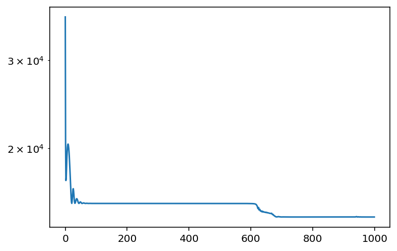
You should notice the first plateau, followed by the second plateau. This corresponds to the two phases of learning.

Now, thus far, we have set up the problem in a fashion that is essentially "trivial". What if, however, we wanted to try fitting a mixture Gaussian where we didn't know exactly how many mixture components there ought to be?

To check that out, head over to the next section in this chapter.