%load_ext autoreload
%autoreload 2
%matplotlib inline
%config InlineBackend.figure_format = 'retina'

Logistic Regression

Logistic regression builds upon linear regression. We use logistic regression to perform binary classification, that is, distinguishing between two classes. Typically, we label one of the classes with the integer 0, and the other class with the integer 1.

What does the model look like? To help you build intuition, let's visualize logistic regression using pictures again.

Matrix Form

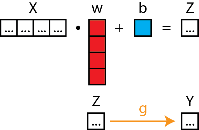
Here is logistic regression in matrix form.

Neural Diagram

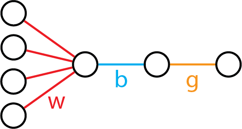
Now, here's logistic regression in a neural diagram:

Interactive Activity

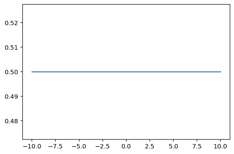
As should be evident from the pictures, logistic regression builds upon linear regression simply by changing the activation function from an "identity" function to a "logistic" function. In the one-dimensional case, it has the same two parameters as one-dimensional linear regression, $w$ and $b$. Let's use an interactive visualization to visualize how the parameters $w$ and $b$ affect the shape of the curve.

(Note: this exercise is best done in a live notebook!)

from dl_workshop.answers import logistic
logistic??

/home/runner/work/dl-workshop/dl-workshop/src/dl_workshop/answers.py:34: TqdmExperimentalWarning: Using `tqdm.autonotebook.tqdm` in notebook mode. Use `tqdm.tqdm` instead to force console mode (e.g. in jupyter console)
  from tqdm.autonotebook import tqdm
WARNING:absl:No GPU/TPU found, falling back to CPU. (Set TF_CPP_MIN_LOG_LEVEL=0 and rerun for more info.)

import jax.numpy as np
import matplotlib.pyplot as plt
from ipywidgets import interact, FloatSlider

@interact(w=FloatSlider(value=0, min=-5, max=5), b=FloatSlider(value=0, min=-5, max=5))
def plot_logistic(w, b):
    x = np.linspace(-10, 10, 1000)
    z = w * x + b  # linear transform on x
    y = logistic(z)    
    plt.plot(x, y)

Parameters of the model

As we can see, there are two parameters $w$ and $b$. For those who may be encountering the model for the first time, this is what each of them control:

• $w$ controls how steep the step function is between 0 and 1 on the y-axis. Its sign also controls whether class 1 is associated with smaller values or larger values.
• $b$ controls the midpoint location of the curve. More negative values of $b$ shift it to the left; more positive values of $b$ shift it to the right.

Make simulated data

Once again, we are going to use simulated data to help us anchor our understanding. Along the way, we will see how logistic regression, once again, fits inside the same framework of "model, loss, optimizer".

import numpy.random as npr

x = np.linspace(-5, 5, 100)
w = 2
b = 1
z = w * x + b + npr.random(size=len(x))
y_true = np.round(logistic(z))
plt.scatter(x, y_true, alpha=0.3);

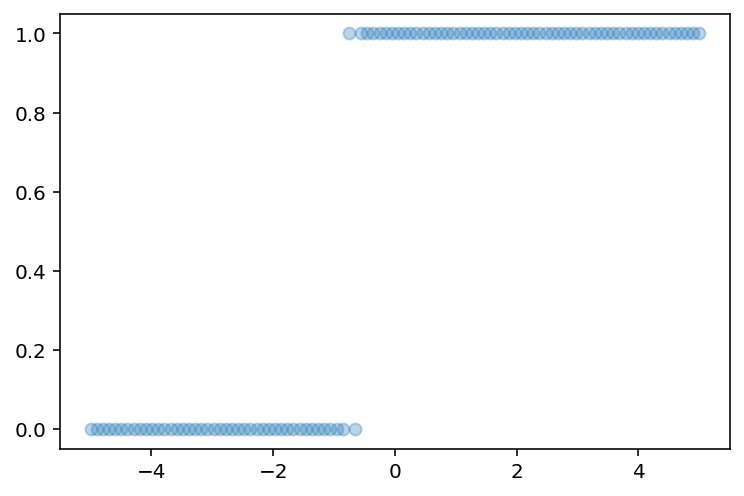
Here, we set $w$ to 2 and $b$ to 1, added some noise in there too, and rounded off the logistic-transformed values to between 0 and 1.

Binary Classification Loss Function

How would we quantify how good or bad our model is? In this case, we use the logistic loss function, also known as the binary cross entropy loss function.

Expressed in equation form, it looks like this:

$$L = -\sum (y \log(p) + (1-y)\log(1-p)$$

Here:

• $y$ is the actual class, namely $1$ or $0$.
• $p$ is the predicted class.

If you're staring at this equation, and thinking that it looks a lot like the Bernoulli distribution log likelihood, you are right!

Discussion

Let's think about the loss function for a moment:

• What happens to the term $y \log(p)$ when $y=0$ and $y=1$? What about the $(1-y)\log(1-p)$ term?
• What happens to both terms when $p \approx 0$ and when $p \approx 1$ (but still bounded between 0 and 1)?

The answers are as follows:

• When $y=0$, $y \log(p) = $, and when $y=1$, $(1-y)\log(1-p) = 0$.
• When $p \rightarrow 0$, then $\log(p)$ approaches negative infinity. Likewise for $\log(1-p)$ when $p \rightarrow 1$

Exercise: Write down the logistic regression model

Using the same patterns as you did before for the linear model, define a function called logistic_model, which accepts parameters theta and data x.

# Exercise: Define logistic model
def logistic_model(theta, x):
    pass

from dl_workshop.answers import logistic_model

Exercise: Write down the logistic loss function

Now, write down the logistic loss function. It is defined as the negative binary cross entropy between the ground truth and the predicted.

The binary cross entropy function is available for you to use:

from dl_workshop.answers import binary_cross_entropy

binary_cross_entropy??

# Exercise: Define logistic loss function
def logistic_loss(params, model, x, y):
    pass

from dl_workshop.answers import logistic_loss
logistic_loss??

Now define the gradient of the loss function, using grad!

from jax import grad
from dl_workshop.answers import dlogistic_loss

# Exercise: Define gradient of loss function.
# dlogistic_loss = ...

Exercise: Initialize logistic regression model parameters using random numbers

Because the parameters are identical to linear regression, you probably can use the same initialize_linear_params function.

from dl_workshop.answers import initialize_linear_params

theta = initialize_linear_params()
theta

{'w': 1.0922641774757724, 'b': -0.1883343121604675}

Exercise: Write the training loop!

This will look very similar to the linear model training loop, because the same two parameters are being optimized. The thing that should change is the loss function and gradient of the loss function.

from dl_workshop.answers import model_optimization_loop

losses, theta = model_optimization_loop(
    theta,
    logistic_model,
    logistic_loss,
    x,
    y_true,
    n_steps=5000,
    step_size=0.0001
)

print(theta)

{'w': DeviceArray(2.5260236, dtype=float32), 'b': DeviceArray(1.4088745, dtype=float32)}

You'll notice that the values are off from the true value. Why is this so? Partly it's because of the noise that we added, and we also rounded off values.

Let's also print out the losses to check that "learning" has happened.

plt.plot(losses);

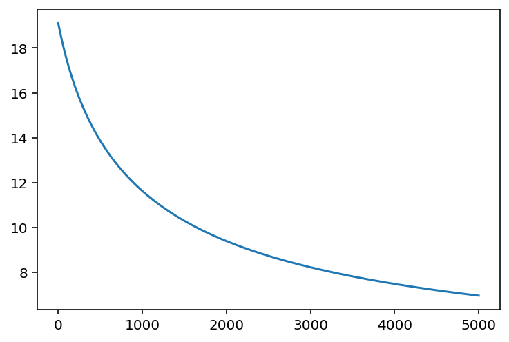
We might argue that the model hasn't yet converged, so we haven't yet figured out the parameters that best explain the data, given the model.

And finally, checking the model against the actual values:

plt.scatter(x, y_true, alpha=0.3)
plt.plot(x, logistic_model(theta, x), color='red');

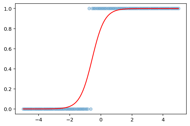
Indeed, we might say that the model parameters could have been optimized further, but as it stands, I'd say we did a pretty good job.

Exercise

What if we did not round off the values, and did not add noise to the original data? Try re-running the model without those two.

Summary

Let's recap what we learned here.

1. We saw that logistic regression is nothing more than a natural extension of linear regression.
2. We saw the introduction of the logistic loss function, and some of its properties.
3. We finally saw that we could optimize a model, leveraging the same grad function from JAX.

To reinforce point 1, let's look at logistic regression in matrix form again.

See how there is an extra function $g$ (in yellow), which is the logistic function, that is tacked on.

To further reinforce the ideas, we should look at the neural diagram once more.

Once again, it's linear model + one more function.

Remember this pattern: it will make neural networks much clearer in the next section!