![]()
%load_ext autoreload
%autoreload 2
%matplotlib inline
%config InlineBackend.figure_format = 'retina'
Applying Dirichlet-processes to mixture-model clustering
Over the previous two sections, we learned about Dirichlet processes and Gaussian Mixture Model-based clustering. In this section, we're going to put the two concepts together!
A data problem with unclear number of modes
Let's start with a data problem that is a bit trickier to solve: one that has multiple numbers of modes, but for which the mixture distribution visually obscures the true number of modes present.
from jax import numpy as np, random, vmap, jit, grad, lax
import matplotlib.pyplot as plt
weights_true = np.array([2, 10, 1, 6])
locs_true = np.array([-2., -5., 3., 8.])
scale_true = np.array([1.1, 2, 1., 1.5,])

base_n_draws = 1000
key = random.PRNGKey(42)
keys = random.split(key, 4)

draws = []
for i in range(4):
    shape = int(base_n_draws * weights_true[i]),
    draw = scale_true[i] * random.normal(keys[i], shape=shape) + locs_true[i]
    draws.append(draw)
data_mixture = np.concatenate(draws)
plt.hist(data_mixture);
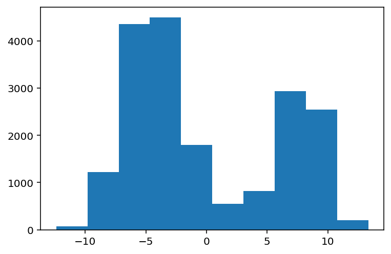
From the histogram, it should be easy to tell that this is not going to be an easy problem to solve. Firstly, the mixture distributions in reality have 4 components. But what we get looks more like 2 components... or really? Could it be that we're lying by using a histogram?
plt.hist(data_mixture, bins=100);
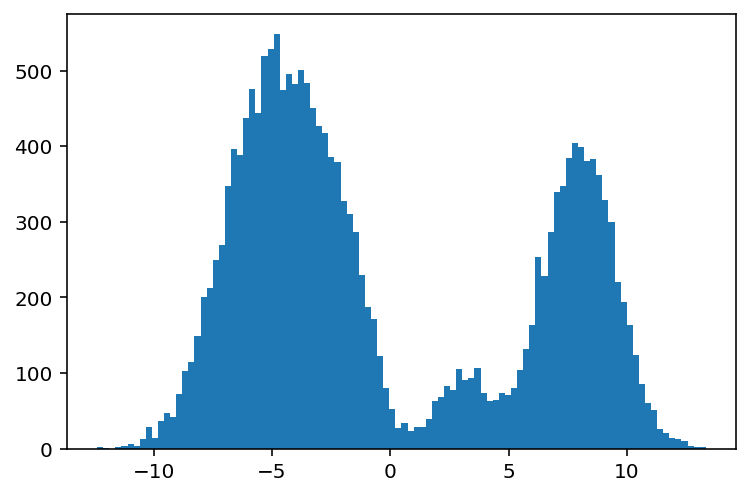
Aha! The case against histograms reveals itself. Turns out there's lots of problems using histograms, and I shan't go deeper into them here, but obscuring data is one of those issues. To learn more, I wrote a blog post on the matter.
In any case, this situation is a clear one where the distribution shape clearly masks the number of mixture components. How can we get around this?
Here, we can turn to Dirichlet processes as a tool to help us. Because DPs don't impose an exact number of significant categories on us, but instead allow us to control their number probabilistically with a single "concentration" parameter, we can instead write down a model to learn the:
- concentration parameters,
- optimal relative weighting of components, conditioned on concentration parameters,
- distribution parameters for each component, conditioned on data.
This effectively forms a Dirichlet-Process Gaussian Mixture Model.
Let's see this in action!
Dirichlet-Process Gaussian Mixture Model (DP-GMM)
The DP-GMM model presumes an infinite (or countably large) number of states, with one Gaussian available per state. The first thing we need to do is to write down the joint log-likelihood of every parameter in our model. As always, before we write down that joint log-likelihood, the first thing we must do is correctly specify what the data generating process is.
Data generating process for a DP-GMM
This could be our data generating process:
- We start with a large number of states, and for each one, their likelihood of ocurring is goverened by a concentration parameter.
- With each state and their corresponding probabilities, we draw a number from the corresponding mixture Gaussian.
- That number's likelihood is proportional to the state from which it was drawn.
With this idea in hand, we can start composing together the joint log-likelihood of the model, conditioned on its parameters and data.
Log-likelihood for the component weights
The first piece we need to compose together is the component weights. We have that already defined!
from dl_workshop.gaussian_mixture import component_probs_loglike

component_probs_loglike??
To quickly recap what this is: it's the log likelihood of a categorical probability vector under a Dirichlet process with a specified concentration parameter.
Log-likelihood for the Gaussian mixture
The second piece we need is the Gaussian mixture log-likelihood.
from dl_workshop.gaussian_mixture import mixture_loglike

mixture_loglike??
And to recap this one really quickly: this is the log likelihood of the observed data under each of the component weights.
Joint log-likelihood
Put together, the joint log-likelihood of the Gaussian mixture model is:
def joint_loglike(
    log_component_weights,
    log_concentration,
    num_components,
    component_mus,
    log_component_scales,
    data
):
    component_probs = np.exp(log_component_weights)
    probs_ll = component_probs_loglike(
        log_component_weights,
        log_concentration,
        num_components
    )

    mix_ll = mixture_loglike(
        log_component_weights,
        component_mus,
        log_component_scales,
        data
    )

    return probs_ll + mix_ll
Through log likelihood function, we are expressing the dependence of the mixture Gaussians on the component probs, and the dependence of the component probs on the concentration parameter.
Optimization
We can now begin optimizing our mixture model parameters.
Loss function
As always, we define the loss function.
def make_joint_loss(num_components):
    def inner(params, data):
        (
            log_component_weights,
            log_concentration,
            component_mus,
            log_component_scales
        ) = params

        ll = joint_loglike(
            log_component_weights,
            log_concentration,
            num_components,
            component_mus,
            log_component_scales,
            data,
        )
        return -ll
    return inner

joint_loss = make_joint_loss(num_components=25)
The closure pattern is here, so that we can set the number of components to use for Dirichlet estimation without making it part of the params to optimize.
Gradient function
We then define the gradient function:
djoint_loss = grad(joint_loss)
Because I know these work, I am going to skip over test-driving them.
Initialization
We'll now start by initializing our parameters.
k1, k2, k3, k4 = random.split(key, 4)
n_components = 50

log_component_weights_init = random.normal(k1, shape=(n_components,))
log_concentration_init = random.normal(k2, shape=(1,))
component_mus_init = random.normal(k3, shape=(n_components,))
log_component_scales_init = random.normal(k4, shape=(n_components,))

params_init = log_component_weights_init, log_concentration_init, component_mus_init, log_component_scales_init
Training Loop
Now we write the training loop, leveraging the functions we had before.
from jax.experimental.optimizers import adam
from dl_workshop.gaussian_mixture import make_step_scannable

adam_init, adam_update, adam_get_params = adam(0.05)
step_scannable = make_step_scannable(
    get_params_func=adam_get_params,
    dloss_func=djoint_loss,
    update_func=adam_update,
    data=data_mixture,
)
step_scannable = jit(step_scannable)
Run training
Finally, we train the model!
from time import time

start = time()
initial_state = adam_init(params_init)
N_STEPS = 10000

final_state, state_history = lax.scan(step_scannable, initial_state, np.arange(N_STEPS))
end = time()
print(f"Time taken: {end - start:.2f} seconds.")
Visualize training
We're going to make the money figure first. Let's visualize the evolution of the mixture Gaussians over training iteration.
params_history = adam_get_params(state_history)
log_component_weights_history, log_concentration_history, component_mus_history, log_component_scales_history = params_history
from dl_workshop.gaussian_mixture import animate_training
%%capture
params_for_plotting = [log_component_weights_history, component_mus_history, log_component_scales_history]
animation = animate_training(params_for_plotting, int(N_STEPS / 200), data_mixture)
from IPython.display import HTML
HTML(animation.to_html5_video())
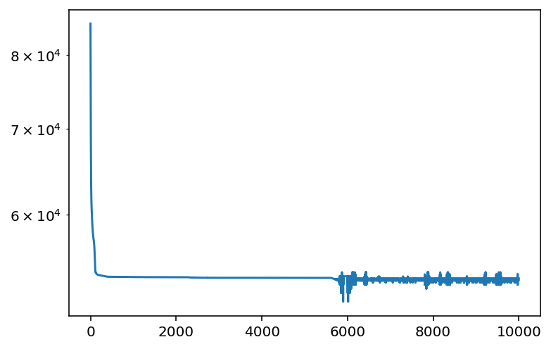
And for the losses:
joint_loss = jit(joint_loss)
losses = []
for w, c, m, s in zip(log_component_weights_history, log_concentration_history, component_mus_history, log_component_scales_history):
    prm = (w, c, m, s)
    l = joint_loss(prm, data_mixture)
    losses.append(l)
plt.plot(losses)
plt.yscale("log")
from dl_workshop.gaussian_mixture import normalize_weights
params_opt = adam_get_params(final_state)
log_component_weights_opt = params_opt[0]
component_weights_opt = np.exp(log_component_weights_opt)
plt.plot(normalize_weights(component_weights_opt), marker="o")
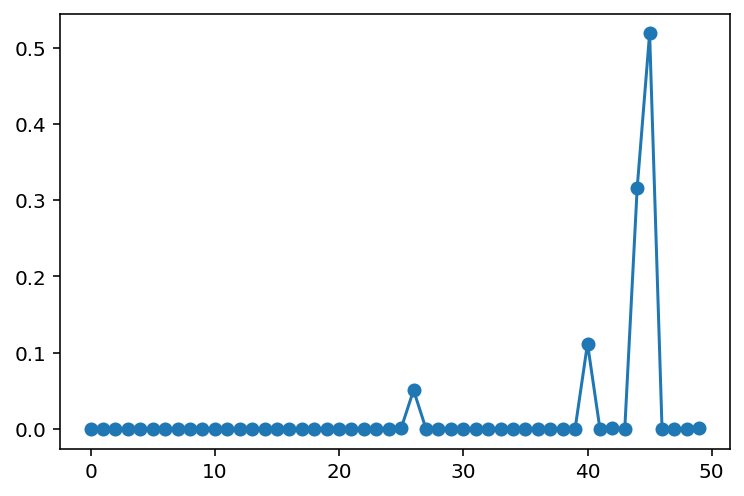
Looks like we are able to recover the major components, in the correct proportions!
If you remembered what the data looked like in 1 dimension, there were basically only 3 majorly-identifiable components. Given enough training iterations (we had to go to 10,000 iterations), our trained model was able to identify all of them, while assigning insignificant probability mass to the rest.
Some caveats
While the main point of this chapter was to show you that it is possible to use gradient-based optimization to cluster data, the same caveats that apply to GMM-based clustering also apply here.
For example, label switching is prominent: the components that are prominent may switch at any time during the gradient descent process. If you observed the video carefully, you would see that in action too. When it comes to MCMC for fully Bayesian inference, this is a problem. With maximum likelihood estimation using gradient descent, however, this is less of an issue, as we usually only end up taking the final optimized parameters.
Summary
The primary purpose of this notebook was to show you that gradient descent is not only for supervised machine learning, but also for unsupervised learning. More generally, gradients can be used anywhere there is an "optimization" problem setup. In this case, identifying clusters of data in a mixture model is a classic unsupervised machine learning problem, but because we cast it in the form of a log-likelihood optimization problem, we were able to leverage gradients to solve this problem.
Aside from that, we saw the JAX idioms in action: vmap, lax.scan, grad, jit and more.
Once again, vmap and lax.scan replaced
many of the for-loops that we might have otherwise written,
grad gave us easy access to gradients,
and jit gave us the advantage of compilation.