%load_ext autoreload
%autoreload 2
%matplotlib inline
%config InlineBackend.figure_format = 'retina'

Neural Networks

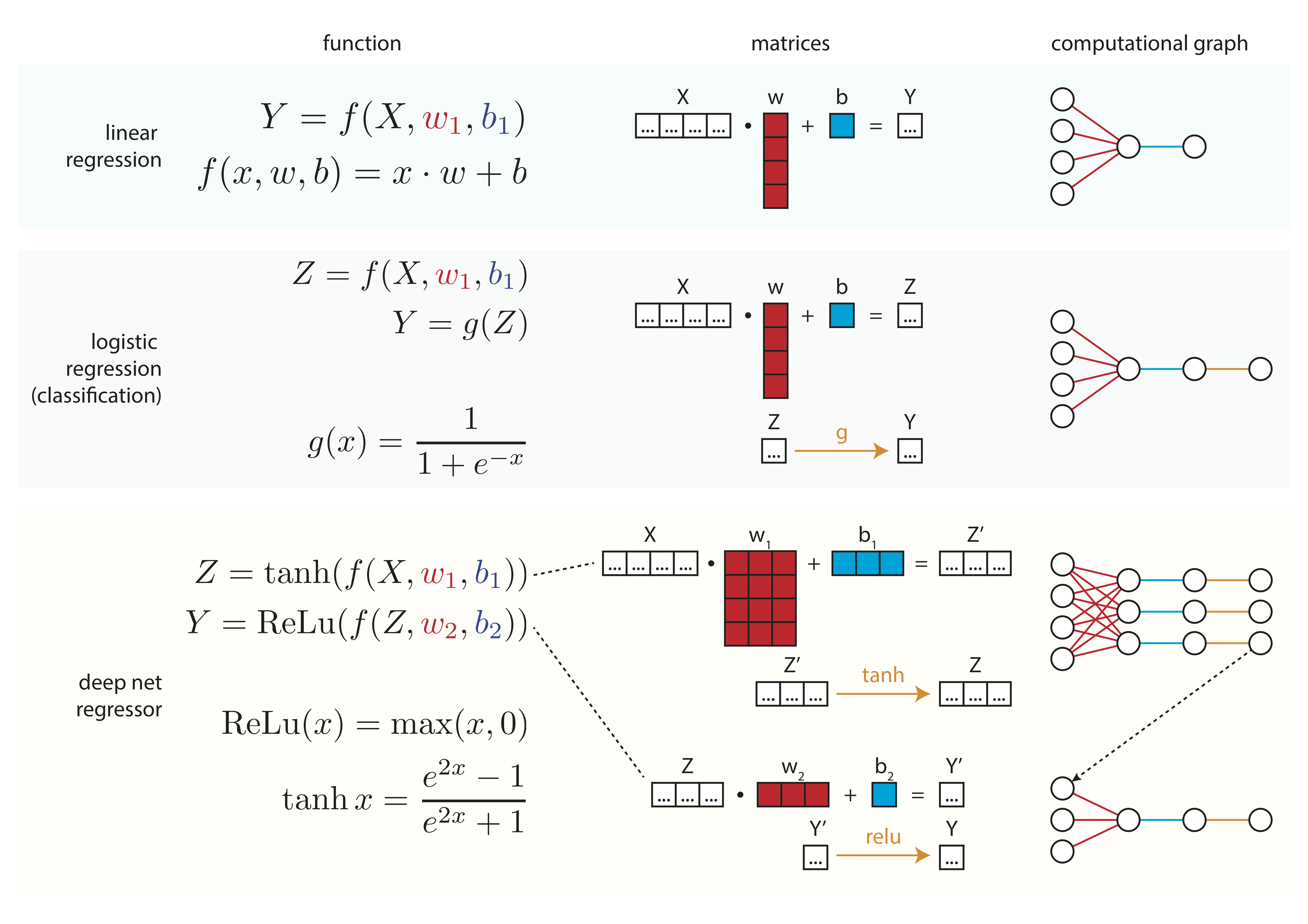
Neural networks are basically very powerful versions of logistic regressions. Like linear and logistic regression, they also take our data and map it to some output, but does so without ever knowing what the true equation form is.

That's all a neural network model is: an arbitrarily powerful model. How do feed forward neural networks look like? To give you an intuition for this, let's see one example of a deep neural network in pictures.

Pictorial form

Matrix diagram

As usual, in a matrix diagram.

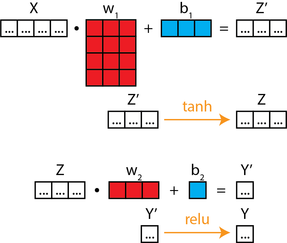
If this looks like a stack of logistic regression-like models, then you're right! This is the essence of what a neural network model is underneath the hood.

Neural diagram

And for correspondence, let's visualize this in a neural diagram.

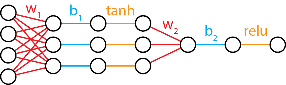
There's some syntax/nomenclature that we need to introduce here.

Notice how $w_1$ reshapes our data to go from 4 inputs to 3 outputs. In neural network lingo, we call the 4 inputs "4 input nodes", and the 3 outputs "3 hidden nodes". If you are familiar with linear algebra operations, you'll know that this operation is a projection of data from 4 dimensions to 3 dimensions.

The second set of weights, $w_2$ , take us from 3 dimensions to 1, and the 1 dimension at the end of the relu function is called the "output node".

The orange functions are called activation functions, and they are a transformation on the linear projection steps (red and blue) that precede them.

We've drawn the computation graph in a very explicit fashion, documenting every math transform in there. However, in the literature, you'll find that most authors omit the blue and orange steps, and instead leave them as implicit in their model illustrations, especially when they have, as a modelling choice, opted for identical activation functions.

Using neural networks on some real data

We are going to try using some real data from the UCI Machine Learning Repository to something related to the work that I am engaged in: predicting molecular properties from molecule descriptors.

With the dataset below, we want to predict whether a compound is biodegradable based on a series of 41 chemical descriptors. This is a classical "classification" problem, where the output is a 1/0 result, much like the logistic regression problem from before.

The dataset was taken from: https://archive.ics.uci.edu/ml/datasets/QSAR+biodegradation#. I have also prepared the data such that it is split into X (the predictors) and Y (the class that we are trying to predict), so that you do not have to worry about manipulating pandas DataFrames.

Let's read in the data.

import pandas as pd
from pyprojroot import here

X = pd.read_csv(here() / 'data/biodeg_X.csv', index_col=0)
y = pd.read_csv(here() / 'data/biodeg_y.csv', index_col=0)

Neural network model definition

Now, let's write a neural network model. The neural network model that we'll design must start with 41 input nodes, because there are 41 input values. As a modelling choice, we might decide to have 1 hidden layer with 20 nodes. Generally, this is arbitrary, but one general rule-of-thumb is to compress the data projection with fewer outputs than inputs. Finally, we must have an output layer with 1 node, as there is only column of data to predict on. Because this is a classification problem, we will use a logistic activation function right at the end.

We'll start by instantiating a bunch of parameters.

from dl_workshop.answers import noise

params = dict()
params['w1'] = noise((41, 20))
params['b1'] = noise((20,))
params['w2'] = noise((20, 1))
params['b2'] = noise((1,))

/home/runner/work/dl-workshop/dl-workshop/src/dl_workshop/answers.py:34: TqdmExperimentalWarning: Using `tqdm.autonotebook.tqdm` in notebook mode. Use `tqdm.tqdm` instead to force console mode (e.g. in jupyter console)
  from tqdm.autonotebook import tqdm
WARNING:absl:No GPU/TPU found, falling back to CPU. (Set TF_CPP_MIN_LOG_LEVEL=0 and rerun for more info.)

Now, let's define the model as a Python function:

import jax.numpy as np
from dl_workshop.answers import logistic

def neural_network_model(theta, x):
    # "a1" is the activation from layer 1
    a1 = np.tanh(np.dot(x, theta['w1']) + theta['b1'])
    # "a2" is the activation from layer 2.
    a2 = logistic(np.dot(a1, theta['w2']) + theta['b2'])
    return a2

Why do we need a "logistic" function at the end, rather than follow what was in the diagram above (relu)? This is because we are doing a classification problem, therefore we must squash the output to be between 0 and 1.

Optimization loop

Now, write the optimization loop! It will look very similar to the optimization loop that we wrote for the logistic regression classification model. The difference here is the model that is used, as well as the initialized set of parameters.

from dl_workshop.answers import model_optimization_loop, logistic_loss

losses, params = model_optimization_loop(
    params, 
    neural_network_model, 
    logistic_loss,
    X.values,
    y.values,
    step_size=0.0001
)

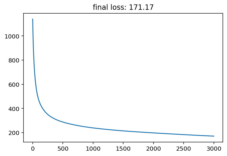
import matplotlib.pyplot as plt

plt.plot(losses)
plt.title(f"final loss: {losses[-1]:.2f}");

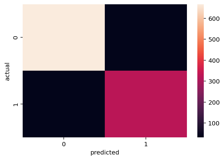
Visualize trained model performance

We can use a confusion matrix to see how "confused" a model was. Read more on Wikipedia.

from sklearn.metrics import confusion_matrix

y_pred = neural_network_model(params, X.values)
confusion_matrix(y, np.round(y_pred))

array([[667,  32],
       [ 33, 323]])

import seaborn as sns

sns.heatmap(confusion_matrix(y, np.round(y_pred)))
plt.xlabel('predicted')
plt.ylabel('actual');

Recap

Deep learning, and more generally any modelling, has the following ingredients:

A model and its associated parameters to be optimized.
A loss function against which we are optimizing parameters.
An optimization routine.

You have seen these three ingredients at play with 3 different models: a linear regression model, a logistic regression model, and a deep feed forward neural network model.

In Pictures

Here is a summary of what we've learned in this tutorial!

Caveats thus far

Deep learning is an active field of research. I have only shown you the basics here. In addition, I have also intentionally omitted certain aspects of machine learning practice, such as

splitting our data into training and testing sets,
performing model selection using cross-validation
tuning hyperparameters, such as trying out optimizers
regularizing the model, using L1/L2 regularization or dropout
etc.

Parting Thoughts

Deep learning is nothing more than optimization of a model with a really large number of parameters.

In its current state, it is not artificial intelligence. You should not be afraid of it; it is nothing more than a really powerful model that maps X to Y.