%load_ext autoreload
%autoreload 2
%matplotlib inline
%config InlineBackend.figure_format = 'retina'

Optimizing Linear Models

What are we optimizing?

In linear regression, we are:

• minimizing (i.e. optimizing) the loss function
• with respect to the linear regression parameters.

Here are the parallels to the example above:

• In the example above, we minimized $f(w)$, the polynomial function. With linear regression, we are minimizing the mean squared error.
• In the example above, we minimized $f(w)$ with respect to $w$, where $w$ is the key parameter of $f$. With linear regression, we minimize mean squared error of our model prediction with respect to the linear regression parameters. (Let's call the parameters collectively $\theta$, such that $\theta = (w, b)$.

Ingredients for "Optimizing" a Model

At this point, we have learned what the ingredients are for optimizing a model:

1. A model, which is a function that maps inputs $x$ to outputs $y$, and its parameters of the model.
   1. Not to belabour the point, but in our linear regression case, this is $w$ and $b$;
   2. Usually, in the literature, we call this parameter set $\theta$, such that $\theta$ encompasses all parameters of the model.
2. Loss function, which tells us how bad our predictions are.
3. Optimization routine, which tells the computer how to adjust the parameter values to minimize the loss function.

Keep note: Because we are optimizing the loss w.r.t. two parameters, finding the $w$ and $b$ coordinates that minimize the loss is like finding the minima of a bowl.

The latter point, which is "how to adjust the parameter values to minimize the loss function", is the key point to understand here.

Writing this in JAX/NumPy

How do we optimize the parameters of our linear regression model using JAX? Let's explore how to do this.

Exercise: Define the linear regression model

Firstly, let's define our model function. Write it out as a Python function, named linear_model, such that the parameters $\theta$ are the first argument, and the data x are the second argument. It should return the model prediction.

What should the data type of $\theta$ be? You can decide, as long as it's a built-in Python data type, or NumPy data type, or some combination of.

# Exercise: Define the model in this function
def linear_model(theta, x):
    pass

from dl_workshop.answers import linear_model

/home/runner/work/dl-workshop/dl-workshop/src/dl_workshop/answers.py:34: TqdmExperimentalWarning: Using `tqdm.autonotebook.tqdm` in notebook mode. Use `tqdm.tqdm` instead to force console mode (e.g. in jupyter console)
  from tqdm.autonotebook import tqdm
WARNING:absl:No GPU/TPU found, falling back to CPU. (Set TF_CPP_MIN_LOG_LEVEL=0 and rerun for more info.)

Exercise: Initialize linear regression model parameters using random numbers

Using a random number generator, such as the numpy.random.normal function, write a function that returns random number starting points for each linear model parameter. Make sure it returns params in the form that are accepted by the linear_model function defined above.

Hint: NumPy's random module (which is distinct from JAX's) has been imported for you in the namespace npr.

def initialize_linear_params():
    pass

# Comment this out if you fill in your answer above.
from dl_workshop.answers import initialize_linear_params
theta = initialize_linear_params()

Exercise: Define the mean squared error loss function with linear model parameters as first argument

Now, define the mean squared error loss function, called mseloss, such that 1. the parameters $\theta$ are accepted as the first argument, 2. model function as the second argument, 3. x as the third argument, 4. y as the fourth argument, and 5. returns a scalar valued result.

This is the function we will be differentiating, and JAX's grad function will take the derivative of the function w.r.t. the first argument. Thus, $\theta$ must be the first argument!

# Differentiable loss function w.r.t. 1st argument
def mseloss(theta, model, x, y):
    pass

from dl_workshop.answers import mseloss

Now, we generate a new function called dmseloss, by calling grad on mseloss! The new function dmseloss will have the exact same signature as mseloss, but will instead return the value of the gradient evaluated at each of the parameters in $\theta$, in the same data structure as $\theta$.

# Put your answer here.


# The actual dmseloss function is also present in the answers,
# but _seriously_, go fill the one-liner to get dmseloss defined!
# If you fill out the one-liner above,
# remember to comment out the answer below
# so that mine doesn't clobber over yours!
from dl_workshop.answers import dmseloss

I've provided an execution of the function below, so that you have an intuition of what's being returned. In my implementation, because theta are passed in as a 2-tuple, the gradients are returned as a 2-tuple as well. The return type will match up with how you pass in the parameters.

from dl_workshop.answers import x, make_y, b_true, w_true

# Create y by replacing my b_true and w_true with whatever you want
y = make_y(x, w_true, b_true)
dmseloss(dict(w=0.3, b=0.5), linear_model, x, y)

{'b': DeviceArray(-39.06814, dtype=float32),
 'w': DeviceArray(-28.964378, dtype=float32)}

Exercise: Write the optimization routine

Finally, write the optimization routine!

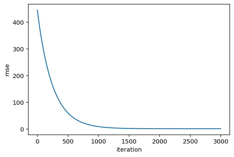
Make it run for 3,000 iterations, and record the loss on each iteration. Don't forget to update your parameters! (How you do so will depend on how you've set up the parameters.)

# Write your optimization routine below.


# And if you implemented your optimization loop,
# feel free to comment out the next two lines
from dl_workshop.answers import model_optimization_loop
losses, theta = model_optimization_loop(theta, linear_model, mseloss, x, y, n_steps=3000)

Now, let's plot the loss score over time. It should be going downwards.

import matplotlib.pyplot as plt

plt.plot(losses)
plt.xlabel('iteration')
plt.ylabel('mse');

Inspect your parameters to see if they've become close to the true values!

print(theta)

{'w': DeviceArray(2.003443, dtype=float32), 'b': DeviceArray(19.98238, dtype=float32)}

Summary

Ingredients of Linear Model

From these first three sections, have seen how the following components play inside a linear model:

1. Model specification ("equations", e.g. $y = wx + b$) and the parameters of the model to be optimized ($w$ and $b$, or more generally, $\theta$).
2. Loss function: tells us how wrong our model parameters are w.r.t. the data ($MSE$)
3. Optimization routine (for-loop)

Let's now explore a few pictorial representations of the model.

Linear Regression In Pictures

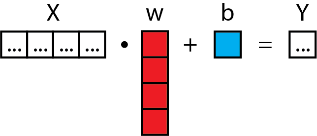
Linear regression can be expressed pictorially, not just in equation form. Here are two ways of visualizing linear regression.

Matrix Form

Linear regression in one dimension looks like this:

Linear regression in higher dimensions looks like this:

This is also known in the statistical world as "multiple linear regression". The general idea, though, should be pretty easy to catch. You can do linear regression that projects any arbitrary number of input dimensions to any arbitrary number of output dimensions.

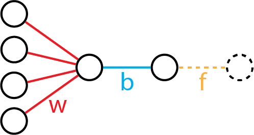
Neural Diagram

We can draw a "neural diagram" based on the matrix view, with the implicit "identity" function included in orange.

The neural diagram is one that we commonly see in the introductions to deep learning. As you can see here, linear regression, when visualized this way, can be conceptually thought of as the baseline model for understanding deep learning.

The neural diagram also expresses the "compute graph" that transforms input variables to output variables.