![]()
%load_ext autoreload
%autoreload 2
%matplotlib inline
%config InlineBackend.figure_format = 'retina'
Writing neural network models using stax
We're now going to try rewriting the neural network model that we had earlier on, now using stax syntax, and traing it using the syntax that we have learned above.
Using stax.serial
Firstly, let's replicate the model using stax.serial. It's a serial composition of a Dense+Tanh layer, followed by a Dense+Sigmoid layer.
from jax.experimental import stax

nn_init, nn_apply = stax.serial(
    stax.Dense(20),
    stax.Tanh,
    stax.Dense(1),
    stax.Sigmoid
)


def nn_init_wrapper(input_shape):
    def inner(key):
        return nn_init(key, input_shape)
    return inner

nn_initializer = nn_init_wrapper(input_shape=(-1, 41))
nn_initializer
Now, we initialize one instance of the parameters.
from jax import random
key = random.PRNGKey(42)
output_shape, params_init = nn_initializer(key)
We'll need a loss funciton to optimize as well.
from jax import grad, numpy as np, vmap
from functools import partial

def binary_cross_entropy(y_true, y_pred, tol=1e-6):
    return y_true * np.log(y_pred + tol) + (1 - y_true) * np.log(1 - y_pred + tol)

def logistic_loss(params, model, x, y):
    preds = vmap(partial(model, params))(x)
    bces = vmap(binary_cross_entropy)(y, preds)
    return -np.sum(bces)

dlogistic_loss = grad(logistic_loss)
Load in data
Now, we load in the data.
import pandas as pd
from pyprojroot import here

X = pd.read_csv(here() / 'data/biodeg_X.csv', index_col=0)
y = pd.read_csv(here() / 'data/biodeg_y.csv', index_col=0)
Test-drive functions to make sure they work
Always important. It'll reveal whether there's anything wrong with our code.
logistic_loss(params_init, nn_apply, X.values, y.values)
Progressively construct our training functions
Firstly, we make sure the step function works with our logistic loss, model func, and actual data.
from jax.experimental.optimizers import adam

adam_init, update, get_params = adam(0.0005)
from dl_workshop.stax_models import step, make_scannable_step, make_training_start
from time import time

stepfunc_nn = partial(step, dlossfunc=dlogistic_loss, get_params=get_params, update=update, model=nn_apply, x=X.values, y_true=y.values)
scannable_step = make_scannable_step(stepfunc_nn)
train_nn = make_training_start(nn_initializer, adam_init, scannable_step, n_steps=3000)
start = time()
final_state, states_history = train_nn(key)
end = time()
print(end - start)
Friends, if you remember where we started in the tutorial.ipynb notebook, the original neural network took approximately a minute to train on a GPU (and longer if on a CPU).
Let's now start by ploting the loss over training iterations. We start first with a function that returns the loss from a given state object.
import matplotlib.pyplot as plt
def calculate_loss(state, get_params, model, lossfunc, x, y):
    params = get_params(state)
    return lossfunc(params, model, x, y)

calculate_loss(final_state, get_params, nn_apply, logistic_loss, X.values, y.values)
Now, we need to vmap it over all states in the states history, to get back the loss score.
calc_loss_vmap = partial(
calculate_loss,
get_params=get_params,
model=nn_apply,
lossfunc=logistic_loss,
x=X.values,
y=y.values
)
start = time()
losses = vmap(calc_loss_vmap)(states_history)
end = time()
print(end - start)
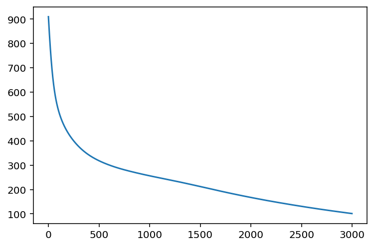
plt.plot(losses)
Training with multiple starting points
Just as above, we can also train the neural network with multiple starting points, again by vmap-ing our training function across split PRNGKeys.
keys = random.split(key, 5)

start = time()
final_states, state_histories = vmap(train_nn)(keys)
end = time()
print(end - start)
get_params(final_states)[0][0].shape
Let's plot the losses over each of the state histories. Our last function calc_loss_vmap calculates loss score for one time point, which we then vmap over a single states_history, so we need another function that encapsulates this behaviour and vmaps over all state histories.
def state_history_loss(state_history):
    losses = vmap(calc_loss_vmap)(state_history)
    return losses

losses = vmap(state_history_loss)(state_histories)
losses.shape
losses
Correctly-shaped! And now plotting it...
plt.plot(losses.T)
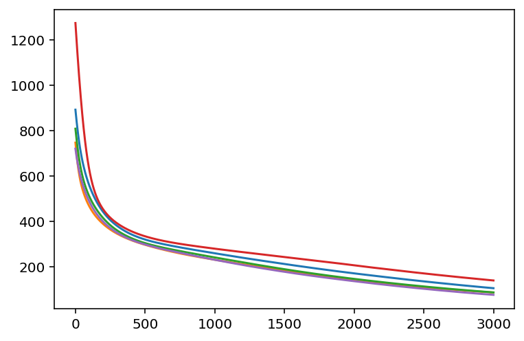
Now that's pretty cool! We were able to see the loss from three independent runs.
With sufficient memory, one would be able to do more runs; when I was writing this notebook early on, I saw that it was getting difficult to do on the order of tens of runs due to memory allocation issues.
Summary
In this notebook, we saw a few things in action.
Firstly, we saw how to use the stax module on a linear model. Anytime we have a new framework for doing differential programming, it's super important to be able to explore it in the context of a linear model, which is basically the foundation of all deep learning.
Secondly, we also explored how to leverage the JAX idioms to create fast parallelized training loops. We mixed-and-matched together jit, vmap, lax.scan, and grad into a performant training loop that was minimally nested.
A corollary of this programming style is that every piece of the code can, in principle, be properly tested, because they are properly isolated. Have you written training loops where you modify a little piece here and a little piece there, until you lost what your original working one looked like? With training functions that are minimally nested, we can control the behaviour explicitly using closures/partials easily. Even when doing experimenation, our code can run reliably and fast.
Thirdly, we saw how to apply the same lessons to training a neural network really fast with multiple starting points. The essence of the solution was to properly structure our program in progressively higher level layers of abstraction. We carefully wrote the program to go from the inner most layer out until we hit our goal of allowing for a set of multiple starts. The key here is that each level of abstraction is very natural, and corresponds to a "unit computation" being applied consistently across an "array" of things. Once we identify that "unit computation", writing the vmap-able or lax.scan-able function becomes very easy.