%load_ext autoreload
%autoreload 2
%matplotlib inline
%config InlineBackend.figure_format = 'retina'

from IPython.display import YouTubeVideo, display

YouTubeVideo("pepAq_dJIik")

Optimized Learning

In this notebook, we will take a look at how to transform our numerical programs into their derivatives.

Autograd to JAX

Before they worked on JAX, there was another Python package called autograd that some of the JAX developers worked on. That was where the original idea of building an automatic differentiation system on top of NumPy started.

Example: Transforming a function into its derivative

Just like vmap, grad takes in a function and transforms it into another function. By default, the returned function from grad is the derivative of the function with respect to the first argument. Let's see an example of it in action using the simple math function:

$$f(x) = 3x + 1$$

# Example 1:
from jax import grad


def func(x):
    return 3 * x + 1


df = grad(func)

# Pass in any float value of x, you should get back 3.0 as the _gradient_.
df(4.0)

WARNING:absl:No GPU/TPU found, falling back to CPU. (Set TF_CPP_MIN_LOG_LEVEL=0 and rerun for more info.)

DeviceArray(3., dtype=float32)

Here's another example using a polynomial function:

$$f(x) = 3x^2 + 4x -3$$

Its derivative function is:

$<span><span class="MathJax_Preview">f'(x) = 6x + 4</span><script type="math/tex">f'(x) = 6x + 4$.

# Example 2:


def polynomial(x):
    return 3 * x ** 2 + 4 * x - 3


dpolynomial = grad(polynomial)

# pass in any float value of x
# the result will be evaluated at 6x + 4,
# which is the gradient of the polynomial function.
dpolynomial(3.0)

DeviceArray(22., dtype=float32)

Using grad to solve minimization problems

Once we have access to the derivative function that we can evaluate, we can use it to solve optimization problems.

Optimization problems are where one wishes to find the maxima or minima of a function. For example, if we take the polynomial function above, we can calculate its derivative function analytically as:

$$f'(x) = 6x + 4$$

At the minima, $f'(x)$ is zero, and solving for the value of $x$, we get $x = -\frac{2}{3}$.

# Example: find the minima of the polynomial function.

start = 3.0
for i in range(200):
    start -= dpolynomial(start) * 0.01
start

DeviceArray(-0.66665125, dtype=float32)

We know from calculus that the sign of the second derivative tells us whether we have a minima or maxima at a point.

Analytically, the second derivative of our polynomial is:

$$f''(x) = 6$$

We can verify that the point is a minima by calling grad again on the derivative function.

ddpolynomial = grad(dpolynomial)

ddpolynomial(start)

DeviceArray(6., dtype=float32)

Grad is composable an arbitrary number of times. You can keep calling grad as many times as you like.

Maximum likelihood estimation

In statistics, maximum likelihood estimation is used to estimate the most likely value of a distribution's parameters. Usually, analytical solutions can be found; however, for difficult cases, we can always fall back on grad.

Let's see this in action. Say we draw 1000 random numbers from a Gaussian with $\mu=-3$ and $\sigma=2$. Our task is to pretend we don't know the actual $\mu$ and $\sigma$ and instead estimate it from the observed data.

from functools import partial

import jax.numpy as np
from jax import random

key = random.PRNGKey(44)
real_mu = -3.0
real_log_sigma = np.log(2.0)  # the real sigma is 2.0

data = random.normal(key, shape=(1000,)) * np.exp(real_log_sigma) + real_mu

Our estimation task will necessitate calculating the total joint log likelihood of our data under a Gaussian model. What we then need to do is to estimate $\mu$ and $\sigma$ that maximizes the log likelihood of observing our data.

Since we have been operating in a function minimization paradigm, we can instead minimize the negative log likelihood.

from jax.scipy.stats import norm


def negloglike(mu, log_sigma, data):
    return -np.sum(norm.logpdf(data, loc=mu, scale=np.exp(log_sigma)))

If you're wondering why we use log_sigma rather than sigma, it is a choice made for practical reasons. When doing optimizations, we can possibly run into negative values, or more generally, values that are "out of bounds" for a parameter. Operating in log-space for a positive-only value allows us to optimize that value in an unbounded space, and we can use the log/exp transformations to bring our parameter into the correct space when necessary.

Whenever doing likelihood calculations, it's always good practice to ensure that we have no NaN issues first. Let's check:

mu = -6.0
log_sigma = np.log(2.0)
negloglike(mu, log_sigma, data)

DeviceArray(3255.0254, dtype=float32)

Now, we can create the gradient function of our negative log likelihood.

But there's a snag! Doesn't grad take the derivative w.r.t. the first argument? We need it w.r.t. two arguments, mu and log_sigma. Well, grad has an argnums argument that we can use to specify with respect to which arguments of the function we wish to take the derivative for.

dnegloglike = grad(negloglike, argnums=(0, 1))

# condition on data
dnegloglike = partial(dnegloglike, data=data)
dnegloglike(mu, log_sigma)

(DeviceArray(-749.3336, dtype=float32), DeviceArray(-2285.8792, dtype=float32))

Now, we can do the gradient descent step!

# gradient descent
for i in range(300):
    dmu, dlog_sigma = dnegloglike(mu, log_sigma)
    mu -= dmu * 0.0001
    log_sigma -= dlog_sigma * 0.0001
mu, np.exp(log_sigma)

(DeviceArray(-3.0087652, dtype=float32), DeviceArray(2.0394986, dtype=float32))

And voila! We have gradient descended our way to the maximum likelihood parameters :).

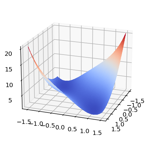
Exercise: Where is the gold? It's at the minima!

We're now going to attempt an exercise. The task here is to program a robot to find the gold in a field that is defined by a math function.

from inspect import getsource

from dl_workshop.jax_idioms import goldfield

print(getsource(goldfield))

def goldfield(x, y):
    """All credit to https://www.analyzemath.com/calculus/multivariable/maxima_minima.html for this function."""
    return (2 * x ** 2) - (4 * x * y) + (y ** 4 + 2)

It should be evident from here that there are two minima in the function. Let's find out where they are.

Firstly, define the gradient function with respect to both x and y. To see how to make grad take a derivative w.r.t. two arguments, see the official tutorial for more information.

from typing import Callable


def grad_ex_1():
    # your answer here
    pass


from dl_workshop.jax_idioms import grad_ex_1

dgoldfield = grad_ex_1()
dgoldfield(3.0, 4.0)

(DeviceArray(-4., dtype=float32), DeviceArray(244., dtype=float32))

Now, implement the optimization loop!

# Start somewhere


def grad_ex_2(x, y, dgoldfield):
    # your answer goes here
    pass


from dl_workshop.jax_idioms import grad_ex_2

grad_ex_2(x=0.1, y=0.1, dgoldfield=dgoldfield)

(DeviceArray(-0.9801416, dtype=float32),
 DeviceArray(-0.9916826, dtype=float32))

Exercise: programming a robot that only moves along one axis

Our robot has had a malfunction, and it now can only flow along one axis. Can you help it find the minima nonetheless?

(This is effectively a problem of finding the partial derivative! You can fix either the x or y to your value of choice.)

def grad_ex_3():
    # your answer goes here
    pass


from dl_workshop.jax_idioms import grad_ex_3

dgoldfield_dx = grad_ex_3()


# Start somewhere and optimize!
x = 0.1
for i in range(300):
    dx = dgoldfield_dx(x)
    x -= dx * 0.01
x

DeviceArray(1.1999948, dtype=float32)

For your reference we have the function plotted below.

import matplotlib.pyplot as plt
from matplotlib import cm

fig, ax = plt.subplots(subplot_kw={"projection": "3d"})

# Change the limits of the x and y plane here if you'd like to see a zoomed out view.
X = np.arange(-1.5, 1.5, 0.01)
Y = np.arange(-1.5, 1.5, 0.01)
X, Y = np.meshgrid(X, Y)
Z = goldfield(X, Y)

# Plot the surface.
surf = ax.plot_surface(
    X,
    Y,
    Z,
    cmap=cm.coolwarm,
    linewidth=0,
    antialiased=False,
)
ax.view_init(elev=20.0, azim=20)