%load_ext autoreload
%autoreload 2
%matplotlib inline
%config InlineBackend.figure_format = 'retina'

Dirichlet Processes: A simulated guide

Introduction

In the previous section, we saw how we could fit a two-component Gaussian mixture model to data that looked like it had just two components. In many real-world settings, though, we oftentimes do not know exactly how many components are present, so one way we can approach the problem is to assume that there are an infinite (or "countably large") number of components available for our model to pick from, but we "guide" our model to focus its attention on only a small number of components provided.

Does that sound magical? It sure did for me when I first heard about this possibility. The key modelling component that we need is a process for creating infinite numbers of mixture weight components from a single controllable parameter, and that naturally gives us a Dirichlet process, which we will look at in this section.

What are Dirichlet processes?

To quote from Wikipedia's article on DPs:

In probability theory, Dirichlet processes (after Peter Gustav Lejeune Dirichlet) are a family of stochastic processes whose realizations are probability distributions.

Hmm, now that doesn't look very concrete. Is there a more concrete way to think about DPs? Turns out, the answer is yes!

At its core, each realization/draw from a DP provides an infinite (or, in computing world, a "large") set of weights that sum to 1. Remember that: A long vector of numbers that sum to 1, which we can interpret as a probability distribution over sets of weights.

Simulating a Dirichlet Process using "stick-breaking"

We're going to look at one way to construct a probability vector, the "stick-breaking" process.

How does it work? At its core, it looks like this, a very simple idea.

1. We take a length 1 stick, draw a probability value from a Beta distribution, break the length 1 stick into two at the point drawn, and record the left side's value.
2. We then take the right side, draw another probability value from a Beta distribution again, break that stick proportionally into two portions at the point drawn, and record the absolute length of the left side's value
3. We then braek the right side again, using the same process.

We repeat this until we have the countably large number of states that we desire.

In code, this looks like a loop with a carryover from the previous iteration, which means it is a lax.scan-able function!

from dl_workshop.gaussian_mixture import stick_breaking_weights
stick_breaking_weights??

As you can see, in the inner function weighting, we first calculate the weight associated with the "left side" of the stick, which we record down and accumulate as the "history" (second tuple element of the return). Our carry is the occupied_probability + weight, which we can use to calculate the length of the right side of the stick (1 - occupied_probability).

Because each beta_i is an i.i.d. draw from beta_draws, we can pre-instantiate a vector of beta_draws and then lax.scan the weighting function over the vector.

Beta distribution crash-course

Because on computers it's hard to deal with infinitely-long arrays, we can instead instantiate a "countably large" array of beta_draws.

Now, the beta_draws, need to be i.i.d. from a source Beta distribution, which has two parameters, a and b, and gives us a continuous distribution over the interval $(0, 1)$. Because of the nature of a and b corresponding to success and failure weights:

• higher a at constant b shifts the distribution closer to 1,
• higher b at constant a shifts the distribution closer to 0,
• higher magnitudes of a and b narrow the distribution width.

Visualizing stick-breaking

For our purposes, we are going to hold a constant at 1.0 while varying b. We'll then see how our weight vectors are generated as a function of b. As you will see, b becomes a "concentration" parameter, which governs how "concentrated" our probability mass is allocated.

Let's see how one draw from a Dirichlet process looks like.

def dp_draw(key, concentration, vector_length):
    beta_draws = random.beta(key=key, a=1, b=concentration, shape=(vector_length,))
    occupied_probability, weights = stick_breaking_weights(beta_draws)
    return occupied_probability, weights

from jax import random
import matplotlib.pyplot as plt

key = random.PRNGKey(42)

occupied_probability, weights = dp_draw(key, 3, 50)
plt.plot(weights)
plt.xlabel("Vector slot")
plt.ylabel("Probability");

WARNING:absl:No GPU/TPU found, falling back to CPU. (Set TF_CPP_MIN_LOG_LEVEL=0 and rerun for more info.)

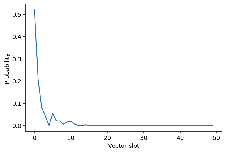
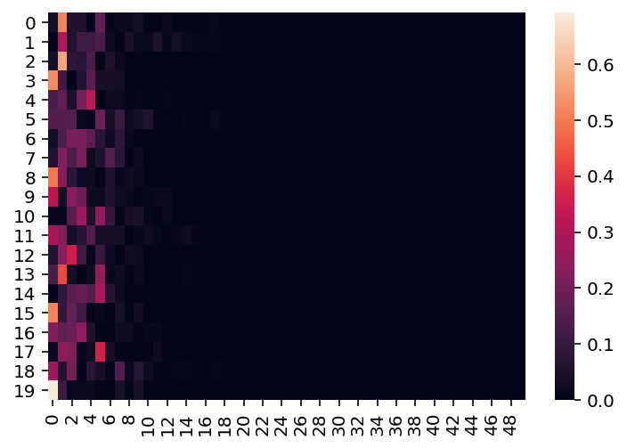
Now, what if we took 20 draws from the Dirichlet process?

To do so, we can vmap dp_draw over split PRNGKeys.

from jax import vmap
from functools import partial
import seaborn as sns
keys = random.split(key, 20)
occupied_probabilities, weights_draws = vmap(partial(dp_draw, concentration=3, vector_length=50))(keys)

sns.heatmap(weights_draws);

Effect of concentration on Dirichlet weights draws

As is visible here, when concentration = 3, most of our probability mass is concentrated across roughly the first 5-8 states.

What happens if we varied the concentration? How does that parameter affect the distribution of weights?

import jax.numpy as np

concentrations = np.array([0.5, 1, 3, 5, 10, 20])

def dirichlet_one_concentration(key, concentration, num_draws):
    keys = random.split(key, num_draws)
    occupied_probabilities, weights_draws = vmap(partial(dp_draw, concentration=concentration, vector_length=50))(keys)
    return occupied_probabilities, weights_draws

keys = random.split(key, len(concentrations))

occupied_probabilities, weights_draws = vmap(partial(dirichlet_one_concentration, num_draws=20))(keys, concentrations)

weights_draws.shape

(6, 20, 50)

fig, axes = plt.subplots(nrows=2, ncols=3, figsize=(3*3, 3*2), sharex=True, sharey=True)

for ax, weights_mat, conc in zip(axes.flatten(), weights_draws, concentrations):
    sns.heatmap(weights_mat, ax=ax)
    ax.set_title(f"Concentration = {conc}")
    ax.set_xlabel("Component")
    ax.set_ylabel("Draw")
plt.tight_layout()

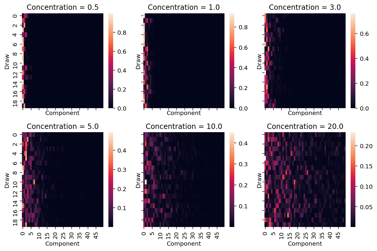
As we increase the concentration value, the probabilities get more diffuse. This is evident from the above heatmaps in the following ways.

1. Over each draw, as we increase the value of the concentration parameter, the probability mass allocated to the components that have significant probability mass decreases.
2. Additionally, more components have "significant" amounts of probability mass allocated.

Running stick-breaking backwards

From this forward process of generating Dirichlet-distributed weights, instead of evaluating the log likelihood of the component weights under a "fixed" Dirichlet distribution prior, we can instead evaluate it under a Dirichlet process with a "concentration" prior. The requirement here is that we be able to recover correctly the i.i.d. Beta draws that generated the Dirichlet process weights.

Let's try that out.

from dl_workshop.gaussian_mixture import beta_draw_from_weights
beta_draw_from_weights??

We essentially run the process backwards, taking advantage of the fact that we know the first weight exactly. Let's try to see how well we can recover the weights.

concentration = 3
beta_draws = random.beta(key=key, a=1, b=concentration, shape=(50,))
occupied_probability, weights = stick_breaking_weights(beta_draws)
final, beta_hat = beta_draw_from_weights(weights)
plt.plot(beta_draws, label="original")
plt.plot(beta_hat, label="inferred")
plt.legend()
plt.xlabel("Component")
plt.ylabel("Beta Draw");

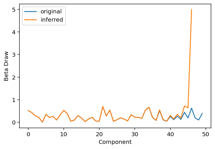
As is visible from the plot above, we were able to recover about 1/2 to 2/3 of the weights before the divergence in the two curves shows up.

One of the difficulties that we have is that when we get back the observed weights in real life, we have no access to how much of the length 1 "stick" is leftover. This, alongside numerical underflow issues arising from small numbers, means we can only use about 1/2 of the drawn weights to recover the Beta-distributed draws from which we can evaluate our log likelihoods.

Evaluating log-likelihood of recovered Beta-distributed weights

So putting things all together, we can take a weights vector, run the stick-breaking process backwards (up to a certain point) to recover Beta-distributed draws that would have generated the weights vector, and then evaluate the log-likelihood of the Beta-disributed draws under a Beta distribution.

Let's see that in action:

from dl_workshop.gaussian_mixture import component_probs_loglike

component_probs_loglike??

And evaluating our draws should give us a scalar likelihood:

component_probs_loglike(np.log(weights), log_concentration=1.0, num_components=25)

DeviceArray(11.000253, dtype=float32)

Log likelihood as a function of concentration

Once again, let's build up our understanding by seeing how the log likelihood of our weights under an assumed Dirichlet process from a Beta distribution changes as we vary the concentration parameter.

log_concentration = np.linspace(-3, 3, 1000)

def make_vmappable_loglike(log_component_probs, num_components):
    def inner(log_concentration):
        return component_probs_loglike(log_component_probs, log_concentration, num_components)
    return inner

component_probs_loglike_vmappable = make_vmappable_loglike(log_component_probs=np.log(weights), num_components=25)

lls = vmap(component_probs_loglike_vmappable)(log_concentration)
plt.plot(log_concentration, lls)
plt.xlabel("Concentration")
plt.ylabel("Log likelihood");

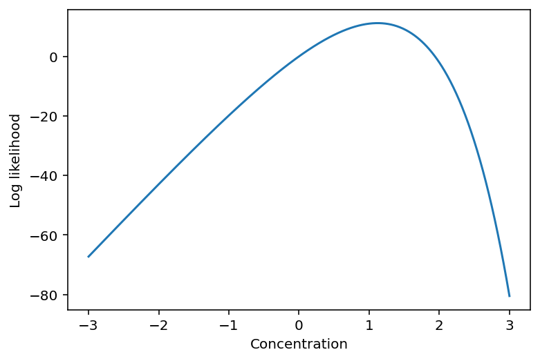
As you can see above, we first constructed the vmappable log-likelihood function using a closure. The shape of the curve tells us that it is an optimizable problem with one optimal point, at least within bounds of possible concentrations that we're interested in.

Optimizing the log-likelihood

Once again, we're going to see how we can use gradient-based optimization to see how we can identify the most likely concentration value that generated a Dirichlet process weights vector.

Define loss function

As always, we start with the loss function definition.

Because our component_probs_loglike function operates only on a single draw, we need a function that will allow us to operate on multiple draws. We can do this by using a closure.

from jax import grad
def make_loss_dp(num_components):
    def loss_dp(log_concentration, log_component_probs):
        """Log-likelihood of component_probabilities of dirichlet process.

        :param log_concentration: Scalar value.
        :param log_component_probs: One or more component probability vectors.
        """
        vm_func = partial(
            component_probs_loglike,
            log_concentration=log_concentration,
            num_components=num_components,
        )
        ll = vmap(vm_func, in_axes=0)(log_component_probs)
        return -np.sum(ll)
    return loss_dp

loss_dp = make_loss_dp(num_components=25)

dloss_dp = grad(loss_dp)

loss_dp(np.log(3), log_component_probs=np.log(weights_draws[3] + 1e-6))

DeviceArray(-353.45496, dtype=float32)

I have opted for a closure pattern here because we are going to require that the Dirichlet-process log likelihood loss function accept log_concentration (parameter to optimize) as the first argument, and log_component_probs (data) as the second. However, we need to specify the number of components we are going to allow for evaluating the Beta-distributed log likelihood, so that goes on the outside.

Moreover, we are assuming i.i.d. draws of weights, therefore, we also vmap over all of the log_component_probs.

Define training loop

Just as with the previous sections, we are going to define the training loops.

from dl_workshop.gaussian_mixture import make_step_scannable

make_step_scannable??

For our demonstration here, we are going to use draws from the weights_draws matrix defined above, specifically the one at index 3, which had a concentration value of 5. Just to remind ourselves what that heatmapt looks like:

sns.heatmap(weights_draws[3]);

Now, we set up the scannable step function:

from jax.experimental.optimizers import adam

adam_init, adam_update, adam_get_params = adam(0.05)

step_scannable = make_step_scannable(
    get_params_func=adam_get_params,
    dloss_func=dloss_dp,
    update_func=adam_update,
    data=np.log(weights_draws[3] + 1e-6), 
)

And then we initialize our parameters

log_concentration_init = random.normal(key)
params_init = log_concentration_init

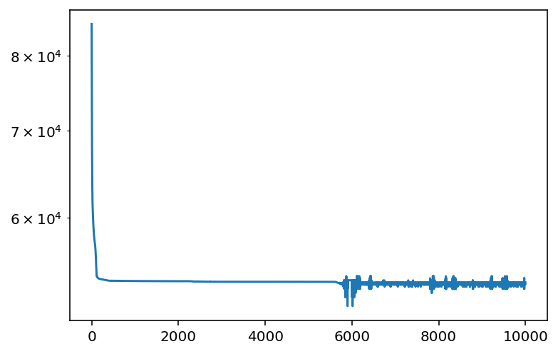
And finally, we run the training loop as a lax.scan function.

from jax import lax

initial_state = adam_init(params_init)

final_state, state_history = lax.scan(step_scannable, initial_state, np.arange(1000))

Now, we can calculate the losses over history.

from dl_workshop.gaussian_mixture import get_loss
get_loss??

from jax import vmap
from functools import partial

losses = vmap(
    partial(
        get_loss, 
        get_params_func=adam_get_params, 
        loss_func=loss_dp, 
        data=np.log(weights_draws[1] + 1e-6)
    )
)(state_history)

plt.plot(losses)

[<matplotlib.lines.Line2D at 0x7f0d2c027f10>]

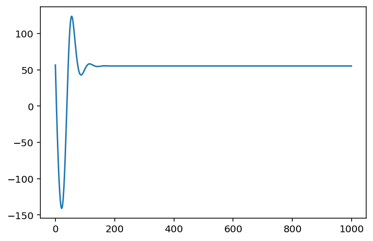
What is the final value that we obtain?

params_opt = adam_get_params(final_state)
params_opt

DeviceArray(1.6304003, dtype=float32)

np.exp(params_opt)

DeviceArray(5.105918, dtype=float32)

This is pretty darn close to what we started with!

Summary

Here, we took a detour through Dirichlet processes to help you get a grounding onto how its math works. Through code, we saw how to:

1. Use the Beta distribution,
2. Write the stick-breaking process using Beta-distributed draws to generate large vectors of weights that correspond to categorical probabilities,
3. Run the stick-breaking process backwards from a vector of categorical probabilities to get back Beta-distributed draws
4. Infer the maximum likelihood concentration value given a set of draws.

The primary purpose of this section was to get you primed for the next section, in which we try to simulatenously infer the number of prominent mixture components and their distribution parameters. A (ahem!) derivative outcome here was that I hopefully showed you how it is possible to use gradient-based optimization on seemingly discrete problems.