![]()
%load_ext autoreload
%autoreload 2
%matplotlib inline
%config InlineBackend.figure_format = 'retina'
from IPython.display import YouTubeVideo, display

YouTubeVideo("6pnl7Eu2wN0")
Eliminating for-loops that have carry-over using lax.scan
We are now going to see how we can eliminate for-loops that have carry-over using lax.scan.
From the JAX docs, lax.scan replaces a for-loop with carry-over,
with some of my own annotations added in for clarity:
Scan a function over leading array axes while carrying along state.
The semantics are described as follows:
def scan(f, init, xs, length=None):
    if xs is None:
         xs = [None] * length
    carry = init
    ys = []
    for x in xs:
        carry, y = f(carry, x)  # carry is the carryover
        ys.append(y)            # the `y`s get accumulated into a stacked array
    return carry, np.stack(ys)
A key requirement of the function f,
which is the function that gets scanned over the array xs,
is that it must have only two positional arguments in there,
one for carry and one for x.
You'll see how we can thus apply functools.partial
to construct functions that have this signature
from other functions that have more arguments present.
Let's see some concrete examples of this in action.
Example: Cumulative Summation
One example where we might use a for-loop is in the cumulative sum or product of an array. Here, we need the current loop information to update the information from the previous loop. Let's see it in action for the cumulative sum:
import jax.numpy as np

a = np.array([1, 2, 3, 5, 7, 11, 13, 17])

result = []
res = 0
for el in a:
    res += el
    result.append(res)
np.array(result)
This is identical to the cumulative sum:
np.cumsum(a)
Now, let's write it using lax.scan, so we can see the pattern in action:
from jax import lax


def cumsum(res, el):
    """
    - `res`: The result from the previous loop.
    - `el`: The current array element.
    """
    res = res + el
    return res, res  # ("carryover", "accumulated")


result_init = 0
final, result = lax.scan(cumsum, result_init, a)
result
As you can see, scanned function has to return two things:
- One object that gets carried over to the next loop (
carryover), and - Another object that gets "accumulated" into an array (
accumulated).
The starting initial value, result_init, is passed into the scanfunc as res on the first call of the scanfunc. On subsequent calls, the first res is passed back into the scanfunc as the new res.
Exercise 1: Simulating compound interest
We can use lax.scan to generate data that simulates
the generation of wealth by compound interest.
Here's an implementation using a plain vanilla for-loop:
wealth_record = []
starting_wealth = 100.0
interest_factor = 1.01
num_timesteps = 100
prev_wealth = starting_wealth

for t in range(num_timesteps):
    new_wealth = prev_wealth * interest_factor
    wealth_record.append(prev_wealth)
    prev_wealth = new_wealth

wealth_record = np.array(wealth_record)
Now, your challenge is to implement it in a lax.scan form.
Implement the wealth_at_time function below.
from functools import partial


def wealth_at_time(prev_wealth, time, interest_factor):
    # The lax.scannable function to compute wealth at a given time.
    # your answer here
    pass


# Comment out the import to test your answer
from dl_workshop.jax_idioms import lax_scan_ex_1 as wealth_at_time

wealth_func = partial(wealth_at_time, interest_factor=interest_factor)
timesteps = np.arange(num_timesteps)
final, result = lax.scan(wealth_func, init=starting_wealth, xs=timesteps)

assert np.allclose(wealth_record, result)
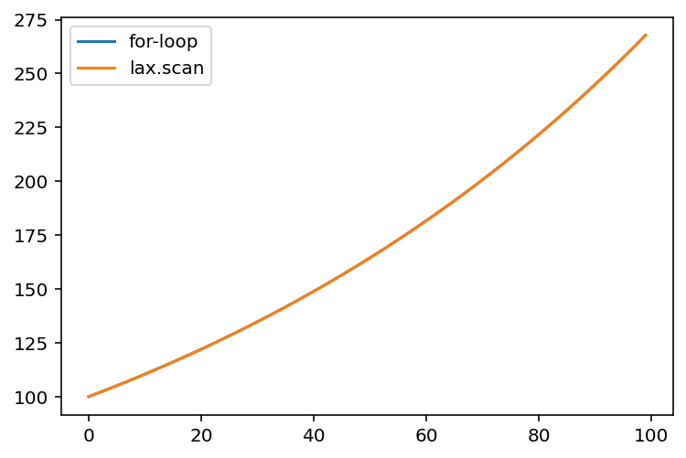
The two are equivalent, so we know we have the lax.scan implementation right.
import matplotlib.pyplot as plt

plt.plot(wealth_record, label="for-loop")
plt.plot(result, label="lax.scan")
plt.legend();
Example: Simulating compound interest from multiple starting points
Previously, was one simulation of wealth generation by compound interest
from one starting amount of money.
Now, let's simulate the wealth generation
for different starting wealth levels;
onemay choose any 300 starting points however one likes.
This will be a demonstration of how to compose lax.scan with vmap
to do computation without loops.
To do so, you'll likely want to start with a function
that accepts a scalar starting wealth
and generates the simulated time series from there,
and then vmap that function across multiple starting points (which is an array itself).
from jax import vmap
def simulate_compound_interest(
starting_wealth: np.ndarray, timesteps: np.ndarray
):
final, result = lax.scan(wealth_func, init=starting_wealth, xs=timesteps)
return final, result
num_timesteps = np.arange(200)
starting_wealths = np.arange(300).astype(float)
simulation_func = partial(simulate_compound_interest, timesteps=np.arange(200))
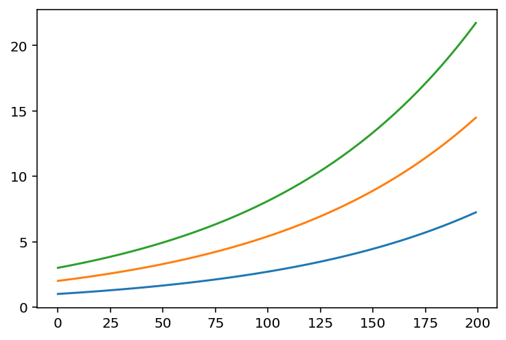
final, growth = vmap(simulation_func)(starting_wealths)
growth.shape
plt.plot(growth[1])
plt.plot(growth[2])
plt.plot(growth[3]);
Exercise 2: Stick breaking process
The stick breaking process is one that is important in Bayesian non-parametric modelling, where we want to model something that may have potentially an infinite number of components while being biased towards a smaller subset of components.
The stick-breaking process uses the following generative process:
- Take a stick of length 1.
- Draw a number between 0 and 1 from a Beta distribution (we will modify this step for this notebook).
- Break that fraction of the stick, and leave it aside in a pile.
- Repeat steps 2 and 3 with the fraction leftover after breaking the stick.
We repeat ad infinitum (in theory) or until a pre-specified large number of stick breaks have happened (in practice).
In the exercise below, your task is to write the stick-breaking process
in terms of a lax.scan operation.
Because we have not yet covered drawing random numbers using JAX,
the breaking fraction will be a fixed variable rather than a random variable.
Here's the vanilla NumPy + Python equivalent for you to reference.
# NumPy equivalent

num_breaks = 30
breaking_fraction = 0.1

sticks = []
stick_length = 1.0
for i in range(num_breaks):
    stick = stick_length * breaking_fraction
    sticks.append(stick)
    stick_length = stick_length - stick
sticks = np.array(sticks)
sticks
def lax_scan_ex_2(num_breaks: int, frac: float):
    # Your answer goes here!
    pass


# Comment out the import if you want to test your answer.
from dl_workshop.jax_idioms import lax_scan_ex_2

sticksres = lax_scan_ex_2(num_breaks, breaking_fraction)
assert np.allclose(sticksres, sticks)